11. Vibrational Polarizability: The Harmonic Oscillator and the Morse Oscillator

Motivation: Nuclear Schrödinger Equation for a Diatomic Molecule

The nuclear Schrödinger equation for a diatomic molecule is

\[ \left(-\frac{\hbar^2}{2M_1}\nabla^2_1 -\frac{\hbar^2}{2M_2}\nabla^2_2 + E_{\text{electronic}}(\mathbf{R}_1,\mathbf{R}_2)\right) \chi(\mathbf{R}_1,\mathbf{R}_2) = E_{\text{total}}\chi(\mathbf{R}_1,\mathbf{R}_2) \]

The potential energy surface on which the nuclei move, \(E_{\text{electronic}}\left(\mathbf{R}_1,\mathbf{R}_2\right)\), depends only on the separation between the molecules,

\[ E_{\text{electronic}}\left(\mathbf{R}_1,\mathbf{R}_2\right) = V\left( \left|\mathbf{R}_1 - \mathbf{R}_2 \right| \right) \]

This suggests changing coordinates using the center of mass. Specifically, we define a coordinate that describes the position of the center of mass

\[ \mathbf{R} = \frac{M_1 \mathbf{R}_1 + M_2\mathbf{R}_2}{M_1 + M_2} \]

and a coordinate that describes the internuclear position

\[ \mathbf{u} = \mathbf{R}_2 - \mathbf{R}_1 \]

To rewrite the Hamiltonian in this new coordinate system, we need to rewrite the kinetic energy in the new coordinates. To do this, notice that differentiation with respect to the old (Cartesian) coordinates of the nuclei can be re-expressed in the new coordinates as:

\[\begin{split} \begin{align} \frac{df}{dX_1} &= \frac{df}{du_x}\frac{du_x}{dX_1} + \frac{df}{dR_x}\frac{dR_x}{dX_1} \\ &= -\frac{df}{du_x} + \frac{M_1}{M_1+M_2}\frac{df}{dR_x} \\ \frac{df}{dX_2} &= \frac{df}{du_x}\frac{du_x}{dX_2} + \frac{df}{dR_x}\frac{dR_x}{dX_2} \\ &= \frac{df}{du_x} + \frac{M_2}{M_1+M_2}\frac{df}{dR_x} \end{align} \end{split}\]

So the momentum operators for the nuclei can be written as:

\[\begin{split} \hat{\mathbf{p}}_1 = -\hat{\mathbf{p}}_u + \frac{M_1}{M_1+M_2}\hat{\mathbf{p}}_R \\ \hat{\mathbf{p}}_2 = \hat{\mathbf{p}}_u + \frac{M_2}{M_1+M_2}\hat{\mathbf{p}}_R \end{split}\]

and the kinetic energy operators are

\[\begin{split} \frac{\hat{\mathbf{p}}_1^2}{2M_1} = \frac{\hat{\mathbf{p}}_u^2}{2M_1} + \frac{M_1\hat{\mathbf{p}}_R^2}{2(M_1+M_2)^2} - \frac{1}{2(M_1+M_2)}\left(\hat{\mathbf{p}}_R \cdot \hat{\mathbf{p}}_u + \hat{\mathbf{p}}_u \cdot \hat{\mathbf{p}}_R\right)\\ \frac{\hat{\mathbf{p}}_2^2}{2M_1} = \frac{\hat{\mathbf{p}}_u^2}{2M_2} + \frac{M_2\hat{\mathbf{p}}_R^2}{2(M_1+M_2)^2} + \frac{1}{2(M_1+M_2)}\left(\hat{\mathbf{p}}_R \cdot \hat{\mathbf{p}}_u + \hat{\mathbf{p}}_u \cdot \hat{\mathbf{p}}_R\right) \end{split}\]

Adding together these expressions gives the Schrödinger equation in the new coordinate system,

\[ \left(-\frac{\hbar^2}{2} \left(\frac{1}{M_1} + \frac{1}{M_2} \right) \nabla^2_u -\frac{\hbar^2}{2} \left(\frac{1}{M_1 + M_2} \right)\nabla^2_R + V(u) \right) \chi(\mathbf{R},\mathbf{u}) = E_{\text{total}}\chi(\mathbf{R},\mathbf{u}) \]

or, introducing the reduced mass

\[\begin{split} \mu = \frac{M_1 M_2}{M_1 + M_2} = \left(\frac{1}{M_1} + \frac{1}{M_2} \right)^{-1} \\ \end{split}\]

and total mass

\[ M = M_1 + M_2 \]

\[ \left(-\frac{\hbar^2}{2 \mu}-\frac{\hbar^2}{2M}\nabla^2_R + V(u) \right) \chi(\mathbf{R},\mathbf{u}) = E_{\text{total}}\chi(\mathbf{R},\mathbf{u}) \]

This Schrödinger equation can be solved by separation of variables. The Schrödinger equation for the center of mass represents the translational motion of the molecule; in the absence of a potential confining the molecule, this is just the Schrödinger equation for a free particle,

\[ -\frac{\hbar^2}{2M}\nabla^2_R \eta(\mathbf{R}) = E \eta(\mathbf{R}) \]

This contributes nothing to the energy if we assume the molecule is not moving (so that its kinetic energy is zero). If the molecule were confined, that confining potential would be inserted here.

The Schrödinger equation for the internuclear coordinate represents the rotations and vibrations of the molecule:

\[ \left(-\frac{\hbar^2}{2 \mu}\nabla_u^2 + V(u) \right) \varphi(\mathbf{u}) = E_{\text{rovib}}\varphi(\mathbf{u}) \]

The Hamiltonian in this equation is typically called the rovibrational Hamiltonian; its energy is the rovibrational energy. Because the potential energy depends only on the internuclear distance, the system is spherically symmetric. Separating out the angular dependence in the usual way,

\[ \left(-\frac{\hbar^2}{2\mu} \left( \frac{d^2}{du^2}+ \frac{2}{u} \frac{d}{du}\right) + \frac{\hat{L}^2(\theta_u,\phi_u)}{2\mu u^2} + V(u) \right) \varphi_{k,J,M_J}(u,\theta_u,\phi_u) = E_{k,J,M_J}\varphi_{k,J,M_J}(u,\theta_u,\phi_u) \]

Recall that \(\hat{L}^2\) is the angular momentum squared, and its eigenfunctions are the spherical harmonics, which we have chosen to denote with a different quantum number to avoid confusion with the electronic problem,

\[\begin{split} \begin{align} \hat{L}^2 Y_J^{M_J}(\theta_u,\phi_u) = \hbar^2 J(J+1) Y_J^{M_J}(\theta_u,\phi_u) \qquad \qquad J&=0,1,2,\ldots \\ M_J &= 0,\pm 1,\ldots\,\pm J \end{align} \end{split}\]

The exact wavefunction is therefore the product of a radial wavefunction and a spherical harmonic,

\[ \varphi_{k,J,M_J}(u,\theta_u,\phi_u) = R_k(u) Y_J^{M_J}(\theta_u,\phi_u) \]

where the radial wavefunction and the rovibrational energy are obtained by solving

\[ \left(-\frac{\hbar^2}{2\mu} \left( \frac{d^2}{du^2}+ \frac{2}{u} \frac{d}{du}\right) + \frac{\hbar^2 J(J+1)}{2\mu u^2} + V(u) \right) R_{k}(u) = E_{k,J}R_{k}(u) \]

Quadratic Approximation to the Potential Energy Curve and the Rigid Rotor Approximation

The potential energy of a diatomic molecule goes to infinity at short internuclear separation (\(u \rightarrow 0\)) because of the nuclear-nuclear repulsion and approaches a constant (which we typically define to be zero) at infinite internuclear distance. In between these limits, there is typically a minimum at \(r_e\), which represents the equilibrium bond length for the molecule (in the absence of quantum effects). If we assume that the atomic nuclei, which are much more massive than electrons, have relatively small De Broglie wavelength and do not deviate far from \(u = r_e\), it is reasonable to expand the potential energy in a Taylor series about that point,

\[ V(u) = V(r_e) + V'(r_e)(u-r_e) + \tfrac{1}{2!}V''(r_e)(u - r_e)^2 + \cdots \]

Because we are expanding around the minimum, \(V'(r_e) = 0\). The term \(V(r_e)\) only shifts the total energy of the system up or down by a constant, so we can choose to set the zero of the energy scale so that \(V(r_e) = 0\). Neglecting higher-order terms in the expansion, which we hope will be small, we can then write

\[ \left(-\frac{\hbar^2}{2\mu} \left( \frac{d^2}{du^2}+ \frac{2}{u} \frac{d}{du}\right) + \frac{\hbar^2 J(J+1)}{2\mu u^2} + \tfrac{1}{2}V''(r_e)(u-r_e)^2 \right) R_{k}(u) = E_{k,J}R_{k}(u) \]

The rotational contribution can also be simplified by taking a Taylor series:

\[ \frac{\hbar^2}{2\mu u^2} = \frac{\hbar^2}{2\mu r_e^2} - \frac{2\hbar^2}{2\mu r_e^3}(u - r_e) + \cdots \]

The first and higher-order terms in the series represent centrifugal distortion, which indicates that a molecule rotates faster and faster, larger bond lengths are favored. Such effects are usually small for low-energy vibrational states of strong bonds, where it is reasonable to make a rigid rotor approximation and truncate the Taylor series after the zeroth order term. The rotational and vibrational problems then decouple, with the rotational wavefunctions and energies being given by:

\[ \frac{\hat{L}^2}{2\mu r_e^2} Y_J^{M_J}(\theta_u,\phi_u) = \frac{\hbar^2 J(J+1)}{2 \mu r_e^2} Y_J^{M_J}(\theta_u,\phi_u) \]

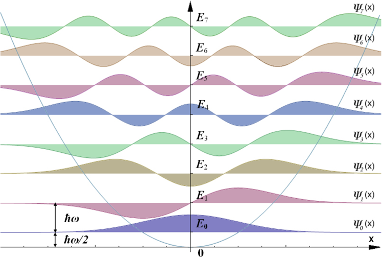
and the vibrational Hamiltonian is then approximated as a quantum mechanical harmonic oscillator:

\[ \left(-\frac{\hbar^2}{2\mu} \left( \frac{d^2}{du^2} + \frac{2}{u} \frac{d}{du}\right) + \tfrac{1}{2}V''(r_e)(u-r_e)^2 \right) R_{k}(u) = E_{k}R_{k}(u) \]

# It's useful to import these libraries. 
# You can import others or not even use these, though.
import numpy as np
import scipy
from scipy import constants

🖩 Exercise: Isotope Effects in Rotational Spectroscopy

For a diatomic molecule that has a permanent dipole moment, allowed rotational transitions correspond to \(\Delta J = \pm 1\).

• A measurement informs you that the transition associated with the \(J=0\) to \(J=1\) transition in \({}^1\text{H}{}^{35}\text{Cl}\) (note the isotope labels) is characterized by \(\tilde{\nu} = \tfrac{1}{\lambda} = 20.9 \text{ cm}^{-1}\). What is the equilibrium bond length of HCl in picometers?

• Assume that \(\text{T}{}^{37}\text{Cl}\) (i.e., \({}^3\text{H}{}^{37}\text{Cl}\)) molecule has the same bond length. What is the wavenumber of the \(J=0\) to \(J=1\) transition for \(\text{T}{}^{37}\text{Cl}\) in \(\text{ cm}^{-1}\)?

Answer:

Let’s start with the second question because it is easier.

The excitation energy is given by the expression

\[ \Delta E = E(J=1) - E(J=0) = \frac{\hbar^2}{2\mu r_e^2}(2) - \frac{\hbar^2}{2\mu r_e^2}(0) = \frac{\hbar^2}{\mu r_e^2} \]

We also know that the wavenumber of the transitions is related to the energy of the transition by

\[ \Delta E = h \nu = \frac{hc}{\lambda} = hc \tilde{\nu} \]

Using the above expression for the change in energy, we see that:

\[ \frac{\Delta E_{{}^1\text{H}{}^{35}\text{Cl}}}{\Delta E_{{}^3\text{H}{}^{37}\text{Cl}}} = \frac{\tilde{\nu}_{{}^1\text{H}{}^{35}\text{Cl}}}{\tilde{\nu}_{{}^3\text{H}{}^{37}\text{Cl}}} = \dfrac{\dfrac{\hbar^2}{\mu_{{}^1\text{H}{}^{35}\text{Cl}} r_e^2}}{\dfrac{\hbar^2}{\mu_{{}^3\text{H}{}^{37}\text{Cl}} r_e^2}} = \frac{\mu_{{}^3\text{H}{}^{37}\text{Cl}}}{\mu_{{}^1\text{H}{}^{35}\text{Cl}}} \]

So:

\[ \tilde{\nu}_{{}^3\text{H}{}^{37}\text{Cl}} = \tilde{\nu}_{{}^1\text{H}{}^{35}\text{Cl}} \left(\frac{\mu_{{}^1\text{H}{}^{35}\text{Cl}}}{\mu_{{}^3\text{H}{}^{37}\text{Cl}}} \right) \]

To a reasonable approximation, we can assume that the masses of these nuclides are integers. (This is true to the number of significant figures given as input.) So:

\[ \tilde{\nu}_{{}^3\text{H}{}^{37}\text{Cl}} = 20.9 \text{cm}^{-1} \left(\frac{\frac{1 \cdot 35}{36}}{\frac{3 \cdot 37}{3+37}}\right) = 20.9 \text{ cm}^{-1} \cdot 0.35035 = 7.32 \text{ cm}^{-1} \]

For part A, we need to use the formula

\[ hc \tilde{\nu} = \Delta E = \frac{\hbar^2}{\mu r_e^2} \]

Rearranging,

\[ r_e^2 = \frac{\hbar^2}{\mu h c \tilde{\nu}} = \frac{(2 \pi)^2 h}{\mu h c \tilde{\nu}} \]

# Report your answers in this cell. I have initialize the variables to None.
re_HCl = None
wavenumber_T37Cl = None

# We start by computing the reduced mass of the species of interest. Use 
mu_H35Cl = (1.00782*34.9688)/(1.00782+34.9688) * scipy.constants.value("atomic mass constant")
mu_T37Cl = (3.01605*36.9659)/(3.01605+36.9659) * scipy.constants.value("atomic mass constant")

# We are given:
wavenumber_H35Cl = 20.9*100 #wavenumber in m^-1
#So (Part B)
wavenumber_T37Cl = wavenumber_H35Cl * mu_H35Cl/mu_T37Cl / 100 #Divide by 100 to get to cm-1

# For Part A, we have the transition energy in Joules
dE_H35Cl = constants.h * constants.c * wavenumber_H35Cl 
# The square of the bond length is. 
re_sq_HCl = constants.hbar**2 / (dE_H35Cl * mu_H35Cl)
# Multiply by 1e12 to get picometers from meters
re_HCl = np.sqrt(re_sq_HCl) * 1e12  

print(f"The equilibrium bond length of HCl is {re_HCl:.1f} pm.")
print(f"The wavenumber of the J=0 -> 1 transition in TCl(37) {wavenumber_T37Cl:.3f} cm-1.")

The equilibrium bond length of HCl is 128.3 pm.
The wavenumber of the J=0 -> 1 transition in TCl(37) 7.342 cm-1.

The Harmonic Oscillator Hamiltonian

It is convenient to change the coordinates in this problem, so that the dependence on \(r_e\) is not explicit. Defining

\[\begin{split} x = u - r_e \\ \kappa_e = V''(r_e) \end{split}\]

the harmonic-oscillator Hamiltonian becomes:

\[ \left(-\frac{\hbar^2}{2\mu} \left( \frac{d^2}{dx^2} + \frac{2}{u} \frac{d}{dx}\right) + \tfrac{1}{2}\kappa_e x^2 \right) R_{k}(x) = E_{k,J}R_{k}(x) \]

In the picture of a diatomic molecule where the atoms are connected to each other with a harmonic spring \(x\) is the deviation of the spring from its equilibrium length and \(\kappa_e\) is the force constant for the spring. The angular frequency for the spring is

\[ \omega = \sqrt{\frac{\kappa_e}{\mu}} \]

and the reduced mass is defined as previously,

\[ \mu = \frac{M_1 M_2}{M_1 + M_2} \]

Solutions to the Harmonic Oscillator Hamiltonian

We will not attempt to solve the harmonic oscillator Schrödinger equation. It suffices to note that the equation is exactly solvable using techniques similar to those we’ve used for other systems, and that the solution is written in terms of (yet another) type of special function, the Hermite polynomials:

\[\begin{split} \begin{align} H_0(y) &= 1 \\ H_1(y) &= 2y \\ H_2(y) &= 4y^2 - 2 \\ H_3(y) &= 8y^3 - 12 \\ H_n(y) &= 2y H_{n-1}(y) - 2(n-1)H_{n-2}(y) \end{align} \end{split}\]

As with the associated Laguerre polynomials, one must be careful because there are (at least) two different definitions of the Hermite polynomials that are prevalent in the literature. These are the-called physicist’s Hermite polynomials. Specifically, we have:

\[ R_k(x) = \sqrt{\frac{1}{2^k k!}}\left(\frac{\mu \omega}{\pi \hbar} \right)^{\frac{1}{4}}H_k\left(x\sqrt{\frac{\mu \omega}{\hbar}}\right) \exp \left[-\frac{1}{2} \left(x\sqrt{\frac{\mu \omega}{\hbar}}\right)^2 \right] \]

and the corresponding eigenvalues are

\[ E_k = \hbar \omega \left( k+ \tfrac{1}{2} \right) = \hbar \sqrt{\frac{\kappa_e}{\mu}} \left( k+ \tfrac{1}{2} \right) \qquad \qquad k=0,1,2,\ldots \]

🖩 Exercise: Isotope Effects in Vibrational Spectroscopy

For a diatomic molecule that is well-described by a harmonic oscillator, allowed vibrational transitions correspond to \(\Delta k = \pm 1\).

• A measurement informs you that the fundamental vibrational transition associated with \(k=0\) to \(k=1\) in \({}^7\text{Li}{}^{7}\text{Li}\) (note the isotope labels) is characterized by \(\tilde{\nu} = \tfrac{1}{\lambda} = 351.43 \text{ cm}^{-1}\). What is the force constant, \(\kappa_e\), for the Lithium dimer in Newton/meter?

• Assume that \({}^6\text{Li}{}^{6}\text{Li}\) molecule has the same force constant. What is the wavenumber of the \(k=0\) to \(k=1\) transition of \({}^6\text{Li}{}^{6}\text{Li}\) in \(\text{cm}^{-1}\)?

Solution:

The energy of the transition is

\[ \Delta E = \hbar \omega = \hbar \sqrt{\frac{\kappa_e}{\mu}} = h c \tilde{\nu} \]

So

\[ \tilde{\nu} = \sqrt{\frac{\kappa_e}{4c^2 \pi^2 \mu}} \]

and

\[ \kappa_e = \frac{h^2 c^2 \tilde{\nu}^2 \mu}{\hbar^2} = 4 \pi^2 c^2 \tilde{\nu}^2 \mu \]

For the second part, we take the ratio of the wavenumbers,

\[ \frac{\tilde{\nu}_{{}^6\text{Li}_2}}{\tilde{\nu}_{{}^7\text{Li}_2}} = \frac{\sqrt{\frac{\kappa_e}{4c^2 \pi^2 \mu_{{}^6\text{Li}_2}}}}{\sqrt{\frac{\kappa_e}{4c^2 \pi^2 \mu_{{}^7\text{Li}_2}}}} = \sqrt{\frac{\mu_{{}^7\text{Li}_2}}{\mu_{{}^6\text{Li}_2}}}=\sqrt{\frac{49\cdot 12 }{36 \cdot 14}}=1.0801 \]

So

\[ \tilde{\nu}_{{}^6\text{Li}_2} = 379.59 \text{ cm}^{-1} \]

# Report your answers in this cell. I have initialize the variables to None.
kappa_e = None                #Force constant in N/m
wavenumber_6Li_2 = None       #wavenumber in cm-1

# We start by computing the reduced mass of the species of interest. Use 
mu_6Li_2 = (6.0151**2)/(2*6.0151) * scipy.constants.value("atomic mass constant")
mu_7Li_2 = (7.0160**2)/(2*7.0160) * scipy.constants.value("atomic mass constant")

# We are given:
wavenumber_7Li_2 = 351.43*100 #wavenumber in m^-1
#So (Part B)
wavenumber_6Li_2 = wavenumber_7Li_2 * np.sqrt(mu_7Li_2/mu_6Li_2) / 100 #Divide by 100 to get to cm-1

# For Part A, we have the transition energy in Joules
dE_7Li_2 = constants.h * constants.c * wavenumber_7Li_2 
# Therefore
sqrt_kappa_e = dE_7Li_2 * np.sqrt(mu_7Li_2) / constants.hbar
# The force constant is
kappa_e = sqrt_kappa_e**2  

print(f"The force constant at equilibrium bond length of the Lithium dimer is {kappa_e:.2f} N/m.")
print(f"The wavenumber of the k=0 -> 1 transition in the Li-6 dimer is {wavenumber_6Li_2:.1f} cm-1.")

The force constant at equilibrium bond length of the Lithium dimer is 25.53 N/m.
The wavenumber of the k=0 -> 1 transition in the Li-6 dimer is 379.5 cm-1.

The Morse Oscillator

Motivation

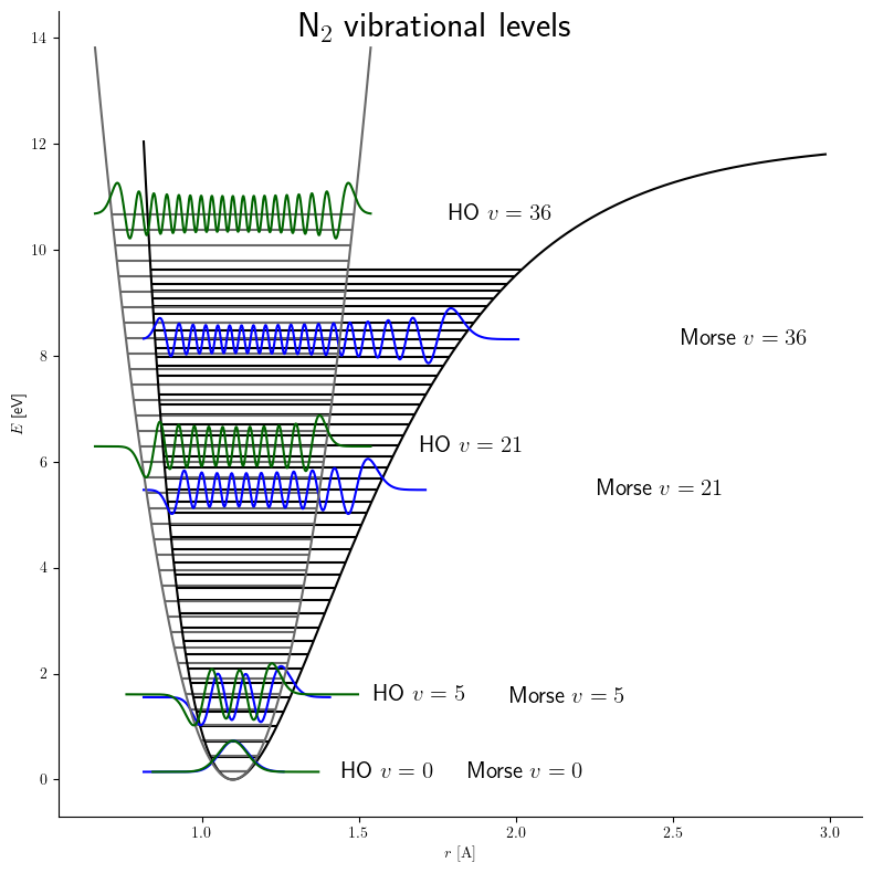
The harmonic oscillator is not very realistic for two reasons

• it predicts that negative bond lengths would be possible, since the potential energy curve does not diverge to infinity as \(u \rightarrow 0\).

• it predicts that chemical bonds never break, since the potential energy curve does not approach an asymptotic constant as \(u \rightarrow \infty\).

The last issue, which is the more severe one from the standpoint of qualitative chemical behavior, can be remedied by replacing the harmonic oscillator potential with the Morse potential,

\[ V_{\text{Morse}}(u) = D_e \left(1 - e^{-a(u-r_e)} \right)^2 \]

Here \(D_e\) is the dissociation constant (the energy it takes to break the bond between the atoms) and \(a\) is related to the force constant by

\[ a = \sqrt{\frac{\kappa_e}{2D_e}} \]

Recall that

\[ \kappa_e = V''_{\text{Morse}}(r_e) \]

Solution

The Schrödinger equation for the Morse potential,

\[ \left(-\frac{\hbar^2}{2\mu} \left( \frac{d^2}{du^2} + \frac{2}{u} \frac{d}{du}\right) + V_{\text{Morse}}(u) \right) \phi_{k}(u) = E_{k}\phi_{k}(u) \]

can also be solved exactly. The eigenfunctions are quite complicated functions of the associated Laguerre polynomials but the energies have a relatively simple expression,

\[ E_k = \hbar \omega_0 \left(k+\tfrac{1}{2}\right) - \frac{\left[ \hbar \omega_0 \left(k+\tfrac{1}{2}\right) \right]^2}{4 D_e} \qquad \qquad k=0,1,2,\ldots,k_{\max} \]

where, just as in the harmonic oscillator,

\[ \omega_0 = a \sqrt{\frac{2D_e}{\mu}} = \sqrt{\frac{\kappa_e}{\mu}} \]

Unlike the harmonic oscillator, only a \(k_{\max} < \infty\) states can be bound by the Morse potential, where

\[ k_{\max} = \left\lfloor \frac{2D_e}{\hbar \omega_0} - \frac{1}{2} \right\rfloor \]

Here \(\lfloor x \rfloor\) denotes the integer part of \(x\). E.g., \(\lfloor 20.3 \rfloor = 20\). The upshot of the equation for \(k_{\max}\) is that the Morse oscillator has about twice as many states with energy less than \(D_e\) as the harmonic oscillator does, because the states of the Morse oscillator become closer and closer together as the molecule gets closer to dissociation. The ability to have only a finite number of bound vibrational states is one way in which the Morse oscillator is more like a real vibrating molecule than the harmonic oscillator.

🖩 Exercise: Compare the Morse and Harmonic Oscillators

A measurement informs you that the fundamental vibrational transition associated with \(k=0\) to \(k=1\) in \({}^7\text{Li}{}^{7}\text{Li}\) (note the isotope labels) is characterized by \(\omega_0 = 6.620\cdot 10^{13} \text{Hz}\). Moreover, the dissociation energy is \(1.6918\cdot 10^{-19} \text{ Joules}\).

• How many bound states does \({}^7\text{Li}_2\) have in the Morse oscillator?

• How many bound states does \({}^6\text{Li}_2\) have in the Morse oscillator? Assume that the Born-Oppenheimer approximation holds.

• What is the zero-point energy of \({}^6\text{Li}_2\) in the harmonic oscillator in Joules?

• What is the zero-point energy of \({}^6\text{Li}_2\) in the Morse oscillator in Joules?

Answer:

This can be seen as a continuation of the previous problem (2.16). Moreover, we realize that the formula for \(\omega_0\) in the Morse oscillator is exactly the same as the formula for \(\omega\) in the harmonic oscillator.

The \(\omega_0\) value for the Li-6 dimer is

\[ \frac{\omega_{0;{{}^6\text{Li}_2}}}{\omega_{0;{{}^7\text{Li}_2}}} = \sqrt{\frac{\mu_{{}^7\text{Li}_2}}{\mu_{{}^6\text{Li}_2}}}=\sqrt{\frac{49\cdot 12 }{36 \cdot 14}}=1.0801 \]

The number of states can be computed relatively easily using the equation

\[ k_{\max} = \left\lfloor \frac{2D_e}{\hbar \omega_0} - 1 \right\rfloor \]

The zero-point energy of the Morse oscillator can be written as a correction to the zero-point energy of the harmonic oscillator. Specifically, using

\[ E_0^{(\text{harmosc})} = \tfrac{1}{2} \hbar \omega_0 \]

one has

\[ E_0^{(\text{Morse})} = E_0^{(\text{harmosc})} - \frac{\left(E_0^{(\text{harmosc})} \right)^2}{4 D_e} \]

# Enter the answers for the variables below. I have initialized the variables to None.
n_boundst_7Li_2 = None       #integer; number of bound states in Li-7 dimer
n_boundst_6Li_2 = None       #integer; number of bound states in Li-6 dimer
zero_pt_6Li_2_Morse = None   #float. zero-point energy in Li-6 dimer in the Morse potential in Joules
zero_pt_6Li_2_harmosc = None #float. zero-point energy in Li-6 dimer in the harmonic oscillator in Joules

# We start by computing the reduced mass of the species of interest. Use 
mu_6Li_2 = (6.0151**2)/(2*6.0151) * scipy.constants.value("atomic mass constant")
mu_7Li_2 = (7.0160**2)/(2*7.0160) * scipy.constants.value("atomic mass constant")

# We are given:
omega0_7Li_2 = 6.620e13 #omega_0 for Li-7 dimer in Hz.
De = 1.6918e-19          #Dissociation energy for Li dimer in Joules.

# Computed omega_0 for the Li-6 dimer in Hz
omega0_6Li_2 = omega0_7Li_2 * np.sqrt(mu_7Li_2/mu_6Li_2)

# Parts A and B
n_boundst_7Li_2 = int(2*De/(constants.hbar*omega0_7Li_2) - 1./2)
n_boundst_6Li_2 = int(2*De/(constants.hbar*omega0_6Li_2) - 1./2)

# Parts D and C
zero_pt_6Li_2_harmosc = constants.hbar*omega0_6Li_2/2
zero_pt_6Li_2_Morse = zero_pt_6Li_2_harmosc - zero_pt_6Li_2_harmosc**2/(4*De)

assert isinstance(n_boundst_7Li_2,int), "Type error: The number of bound states should be an integer."
assert isinstance(n_boundst_6Li_2,int), "Type error: The number of bound states should be an integer."

print(f"The number of bound states in the Morse oscillator for the Li-7 dimer is {n_boundst_7Li_2}.")
print(f"The number of bound states in the Morse oscillator for the Li-6 dimer is {n_boundst_6Li_2}.")
print(f"The zero-point energy of the Morse oscillator for the Li-6 dimer is {zero_pt_6Li_2_Morse:.3e} Joules.")
print(f"The zero-point energy of the harmonic oscillator for the Li-6 dimer is {zero_pt_6Li_2_harmosc:.3e} Joules.")

### BEGIN HIDDEN TESTS
assert(n_boundst_7Li_2 == 47)
assert(n_boundst_6Li_2 == 44)
assert(np.isclose(zero_pt_6Li_2_Morse,3.749e-21,rtol=1e-3))
assert(np.isclose(zero_pt_6Li_2_harmosc,3.770e-21,rtol=1e-3))
### END HIDDEN TESTS

The number of bound states in the Morse oscillator for the Li-7 dimer is 47.
The number of bound states in the Morse oscillator for the Li-6 dimer is 44.
The zero-point energy of the Morse oscillator for the Li-6 dimer is 3.749e-21 Joules.
The zero-point energy of the harmonic oscillator for the Li-6 dimer is 3.770e-21 Joules.

Vibrating Diatomic Molecules in an External Field

Motivation

For polar diatomic molecules, their dipole moment may be approximated as:

\[ \mathbf{p} = q \left(\mathbf{R}_2 - \mathbf{R}_1 \right) \]

where \(q\) is the magnitude of the charges on the atoms and \(\mathbf{R}_2\) is the positively charged atom. The energy of a polar diatomic molecule interacting with an electric field is then

\[ V_{\text{dipole}} = -\mathbf{p} \cdot \mathbf{E} \]

This energy is minimized when the dipole aligns in the field, giving an energy lowering that is proportional to the product of the magnitude of the dipole moment and the electric field strength,

\[ V_{\text{dipole}} = -|\mathbf{p}| |\mathbf{E}| = - q u F \]

where \(q\) is the atomic charge, \(u\) is the internuclear distance, and F is the field strength. This is a quite simple model, and neglects the following

• atomic charges change when the bond length changes

• atoms are not simply point charges

• a molecule’s electrons rearrange in response to the electric field. To a first approximation, this means that the atomic charges change in the presence of the field.

Nonetheless, this model does capture some key features, notably the fact that in the presence of a uniform external field, the bond in a polar diatomic molecule tends to elongate.

Hamiltonian for a Polar Diatomic Molecule in an External Uniform Electric Field

The Hamiltonian for a vibrating molecule in an electric field can then be approximated as

\[ \left(-\frac{\hbar^2}{2\mu} \left( \frac{d^2}{du^2} + \frac{2}{u} \frac{d}{du}\right) + V(u) - q_e u F \right) R_{k}(u) = E_{k}R_{k}(u) \]

where \(q_e\) is magnitude of the atomic charge for \(u = r_e\). If the equilibrium dipole moment of the molecule is known, then

\[ q_e = \frac{\left[\text{dipole moment in Debye}\right] \cdot 3.33564 \cdot 10^{-30} \text{ C/m}}{\text{bond length in meters}} \text{ Coulombs} \]

or, in terms of the charge on the electron \(e\),

\[ q_e = \frac{\left[\text{dipole moment in Debye}\right] \cdot 2.08919 \cdot 10^{-11} e/\text{m}}{\text{bond length in meters}} e \]

The most interesting effects are not those that are associated with the classical interaction energy of the dipole with the field, we usually subtract that energy from the Hamiltonian, so that we only see the change in the molecule’s energy that was induced by the field. I.e., we usually focus on the vibrational dipole polarization energy,

\[ E_k^{(\text{polarization})}(F) = E_k(F) - \left[ E_k(F=0) - q_e r_e F \right] \]

The vibrational dipole polarization energy can be computed from the shifted Schrödinger equation, where

\[\begin{split} \begin{align} \left(-\frac{\hbar^2}{2\mu} \left( \frac{d^2}{du^2}+ \frac{2}{u} \frac{d}{du}\right) + V(u) - q_e (u-r_e) F \right) \psi_{k}(u) &= \left(E_k(F=0) + E_{k}^{(\text{polarization})}(F)\right)\psi_{k}(u) \\ &= E_{k}^{(\text{shifted})}(F)\psi_{k}(u) \end{align} \end{split}\]

where we have (re)defined the energy as

\[ E_k^{(\text{shifted})}(F) = E_k(0) + E_k^{(\text{polarization})}(F) \]

The total energy of the vibrating diatomic molecule can then be expressed as:

\[ E_k(F) = E_k(0) - q_e r_e F + E_k^{(\text{polarization})}(F) \]

If one expands the vibrational polarization energy in a Taylor series,

\[ E_k^{(\text{polarization})}(F) = -\tfrac{1}{2} \alpha_{\text{vib}} F^2 - \tfrac{1}{3!} \beta_{\text{vib}} F^3 - \tfrac{1}{4!} \gamma_{\text{vib}} F^3 + \cdots \]

where \(\alpha_{\text{vib}}\) is the vibrational contribution to the dipole polarizability (subject to the approximations mentioned above) and the higher-order coefficients are the first-, \(\beta\), and higher-order vibrational dipole hyperpolarizabilities.

The Harmonic Oscillator in a Uniform External Electric Field

To model a diatomic molecule vibrating in a uniform electric field, we need to choose a practical model for the vibrational potential energy function, \(V(u)\). The simplest possible model is to use a Harmonic Oscillator, which leads to the Hamiltonian:

\[ \left(-\frac{\hbar^2}{2\mu} \left( \frac{d^2}{du^2} + \frac{2}{u} \frac{d}{du}\right) + \tfrac{1}{2}\kappa_e(u-r_e)^2 - q_e (u-r_e) F \right) R_{k}(u) = E_{k}^{\text{shifted}}(F) R_{k}(u) \]

Sketch of Perturbative Approach

One could treat this Hamiltonian with perturbation theory. By construction, \(E_k^{(\text{shifted})}\) does not depend on the field to first order. Therefore, the leading-order term is the second-order contribution,

\[\begin{split} \left[\frac{d^2 E_k}{dF^2}\right]_{F=0} =\left[\frac{d^2E_k^{(\text{polarization})}}{dF^2}\right]_{F=0}=\left[\frac{d^2E_k^{(\text{shifted})}}{dF^2}\right]_{F=0} = 2q_e \sum_{j=0\\j \ne k}^{\infty}\frac{ \left|\langle R_j(0) | u-r_e |R_k(0) \rangle \right|^2}{E_k(F=0) - E_j(F=0)} \end{split}\]

Evaluating this expression is feasible because the integrals that one needs,

\[ V_{kl} = \int_{-\infty}^{\infty} R_k(u)(u-r_e) R_l(u) du \]

have a simple explicit formulae. Specifically,

\[\begin{split} V_{kl} = \begin{cases} \sqrt{\frac{k}{2}} & k=l+1 \\ \sqrt{\frac{k+1}{2}} & k=l-1 \\ 0 & \text{otherwise} \end{cases} \end{split}\]

Exact Solution by Completing the Square

While a perturbative approach is possible, the harmonic oscillator in a uniform external electric field can be solved exactly. Completing the square on the potential,

\[ \tfrac{1}{2}\kappa_e(u-r_e)^2 - q_e (u-r_e) F = \tfrac{1}{2}\kappa_e\left(u - r_e - \frac{qF}{\kappa_e}\right)^2 - \frac{q^2F^2}{2 \kappa_e} \]

The force constant in this new shifted harmonic oscillator is the still \(\kappa_e\), but the bond length

\[ r_e(F) = r_e + \frac{qF}{\kappa_e} \]

and the energies

\[ E_k^{\text{shifted}}(F) = \hbar \sqrt{\frac{\kappa_e}{\mu}}\left(k+\frac{1}{2}\right) - \frac{q^2F^2}{2 \kappa_e} \]

have chagned. Referring to the definitions above, the vibrational polarization energy is:

\[ E_k^{\text{polarization}}(F) = - \frac{q^2}{2 \kappa_e}F^2 \]

the vibrational polarizability is

\[ \alpha_{\text{vib}} = \frac{q^2}{\kappa_e} \]

and the total vibrational energy of the diatomic molecule in the field

\[ E_k(F) = \hbar \sqrt{\frac{\kappa_e}{\mu}}\left(k+\frac{1}{2}\right) - q r_e F- \frac{q^2}{2 \kappa_e}F^2 \]

🖩 Exercise: Model the HF molecule in a uniform electric field in the Harmonic Oscillator Approximation.

For the \({}^{1}\text{H}{}^{19}\text{F}\) molecule, \(\mu = 6.361 \cdot 10^{-25} \text{ kg}\), \(\kappa_e = 920 \text{ N/m} \), and \(r_e = 91.68 \text{ pm}\). The dipole moment of HF is 1.91 Debye, which corresponds to a semi-reasonable charge of 0.44 \(e\) on the hydrogen atom. Assume the electric field is 1,000,000 V/m.

• How much does the bond elongate in the presence of the external electric field? Report your answer in picometers.

• What value would you obtain if you used second-order perturbation theory to estimate the vibrational polarization energy, \(E_k^{(\text{polarization})}\). Report your answer in Joules.

Hint: Results from the previous block of the notebook may be helpful.

Solution:

This is mostly a pretty straightforward “calculator” exercise. The only tricky part is the use of perturbation theory. However, note that the exact expression has only terms that are linear and quadratic in F. That means that second-order perturbation theory is exact. So you did not need to use perturbation theory. Even if you did, only one state would contribute, so the problem is pretty easy…..

# Report your answers in the variables below, which I have initialized to None.
re_shift = None
e_polarization = None

charge_H = 1.91*3.33564e-30/91.68e-12   #Charge on the hydrogen in Coulombs
field = 1.0e6
kappa_e = 920 
mu = 6.361e-25
re = 91.68e-12

re_shift = charge_H * field / kappa_e * 1e12           #multiply by 1e12 to get units of picometers.
e_polarization = -1 * charge_H**2 * field **2 / (2 * kappa_e)
e_shifted = constants.hbar * np.sqrt(kappa_e/mu) + e_polarization
e_true = e_shifted - charge_H * field * re

print(f"The bond length of HF elongates by {re_shift:.3e} pm in a field of 1,000,000 V/m.")
print(f"The zero-point energy HF changes by {e_polarization:.3e} J in a field of 1,000,000 V/m.")

The bond length of HF elongates by 7.554e-05 pm in a field of 1,000,000 V/m.
The zero-point energy HF changes by -2.625e-30 J in a field of 1,000,000 V/m.

The Morse Oscillator in an External Electric Field

Instead of using a harmonic oscillator to describe the vibrational motion of a polar diatomic molecule, one could use the Morse Oscillator. In this case, the Schrödinger equation is:

\[\begin{split} \begin{align} \left(-\frac{\hbar^2}{2\mu} \left( \frac{d^2}{du^2} + \frac{2}{u} \frac{d}{du}\right) + V_{\text{Morse}}(u) - q_e (u-r_e) F \right) \phi_{k}(u) &= \left(E_k(F=0) + E_{k}^{(\text{polarization})}(F)\right)\phi_{k}(u) \\ &= E_{k}^{(\text{shifted})}(F)\phi_{k}(u) \end{align} \end{split}\]

Unlike the harmonic oscillator in an electric field, it is no longer possible to solve this system exactly. However, there are many possible ways to approximate the energy of a Morse oscillator in a uniform electric field, among them:

• Use the harmonic-oscillator in an external field as a zeroth-order Hamiltonian, and use perturbation theory to estimate the change in energy associated with using the Morse potential instead.

• Use the eigenfunctions of the harmonic oscillator in an electric field as a basis; expand the eigenfunctions of the Morse potential in an electric field in this basis.

• Use the Morse potential without an electric field as a zeroth-order Hamiltonian; use perturbation theory to estimate the effects of the electric field.

• Use the eigenfunctions of the Morse potential without an electric field as a basis; expand the eigenfunctions of the Morse potential in an electric field in this basis.

The first two approaches are arguably preferable mathematically, but the latter two are easier. This is because the matrix elements for the Morse potential in an electric field,

\[ V_{mn} = \int_{-\infty}^{\infty} \phi_m(u;F=0) (u - r_e) \phi_n(u;F=0) du \]

are (relatively) easy to evaluate. Specifically we have:

\[ V_{m<n} = \frac{-1^{m-n+1}}{a(n-m)(2\lambda-n-m-1)}\left[\frac{n! \Gamma(2\lambda - n)(2\lambda - 2n - 1)(2\lambda - 2m - 1)}{m! \Gamma(2\lambda - m)} \right]^{\frac{1}{2}} \]

In practice, this equation is numerically ill-conditioned when \(m\), \(n\), or \(\lambda\) is large, because then some of the terms are gigantic. It is reasonable to cut off the expansion for large \(m\) and large \(n\); when \(\lambda\) is large, one can use the Ramanujan expression for the \(\Gamma\) function,

\[ \Gamma(y) = \sqrt{\pi} \left(\frac{y-1}{e} \right)^{y-1} \left(8(y-1)^3 + 4(y-1)^2 + (y-1) + \frac{1}{30} \right)^{\frac{1}{6}} \]

to evaluate the square root of the ratio of the \(\Gamma\) functions directly

\[ \frac{\Gamma(y)}{\Gamma(x)} = \left(\sqrt{\frac{y-1}{x-1}}\right)^{y-1} \left(\sqrt{\frac{e}{x-1}} \right)^{x-y} \left(\frac{8(y-1)^3 + 4(y-1)^2 + (y-1) + \frac{1}{30}}{8(x-1)^3 + 4(x-1)^2 + (x-1) + \frac{1}{30}}\right)^{\frac{1}{12}} \]

The code below actually uses the (more complicted) Stirling expansion, because in practice it seemed more accurate.

The diagonal elements are:

\[ V_{mm} \approx \frac{\frac{3}{2} + 3m + \frac{13/12 + (7/2)(m^2+m)}{2 \lambda} + \frac{(m+1)^4}{4\lambda^2}}{2\lambda a} \]

In these expressions,

\[ \lambda = \frac{\sqrt{2 \mu D_e}}{a \hbar} \]

Using the aforementioned definition of \(a\),

\[ a = \sqrt{\frac{\kappa_e}{2D_e}} \]

this simplifies to

\[ \lambda = \frac{2 D_e}{\hbar}\frac{\mu}{\kappa_e} = \frac{2 D_e}{\hbar \omega_0} \]

Note. Technically in both perturbation theory and in a variational approach one would need to consider the continuum states, corresponding to the states of the dissociated diatomic molecule. We are neglecting that tricky business here, but that is the main reason that an approach starting from the harmonic oscillator is mathematically preferable.

Note. The choice of \(u = |\mathbf{R}_1 - \mathbf{R}_2|\) or \(u = |\mathbf{R}_2 - \mathbf{R}_1|\) is arbitrary. This means, in practice, that whether one chooses a field oriented in the \(+u\) or \(-u\) direction is arbitrary. One should compute both choices, and pick the one which stabilizes the molecule more. For a Morse oscillator, this corresponds to a field with a negative sign.

👩🏽‍💻 Exercise: Model the HF molecule in a uniform electric field using the Morse potential.

For the \({}^{1}\text{H}{}^{19}\text{F}\) molecule, \(\mu = 6.361 \cdot 10^{-25} \text{ kg}\), \(\kappa_e = 920 \text{ N/m} \), \(D_e = 9.402 \cdot 10^{-19} J\), and \(r_e = 91.68 \text{ pm}\). The dipole moment of HF is 1.91 Debye, which corresponds to a semi-reasonable charge of 0.44 \(e\) on the hydrogen atom. Assume the electric field is 1,000,000 V/m.

Using the integrals provided below, compute the vibrational polarization energy, \(E_{k}^{(\text{polarization})}(F)\), for the Morse Oscillator in a field using perturbation theory and/or basis-set expansion.

1. Compute both first and second-order corrections to the polarization energy if you use perturbation theory. Note that in this case, the first-order contribution to the polarization energy is not exactly zero.

2. Summing over all bound states or using all bound states in the basis is not practical, but you should be sure to not use unbound states.

Given how complicated this is, it is possible that my code below has some mistakes. I’m looking to test whether your code works well assuming that my matrix elements \(V_{mn}\), are coded correctly.

# I've initialized key variables to None. These quantities are printed in the next cell.
epol_pt = None    #Energy of polarization computed using first and second-order perturbation theory, 
                  #    in Joules
epol_basis = None #Energy of polarization computed using basis-set expansion, in Joules

# The below code provides key quantities that are needed for this treatment. 
# All inputs are assumed to be in SI units.

from scipy.linalg import eigh
from scipy.special import gamma,factorial
import math

def Ramanujan_ratio(x,m,n):
    """Computes (Gamma(2x-n)/Gamma(2x-m))^(1/2) using the Ramanujan approximation to the Gamma function"""
    ratio = np.sqrt((2*x-m-1)**(m+1))/np.sqrt((2*x-n-1)**(n+1)) \
            * (cubic_poly(2*x-n-1)/cubic_poly(2*x-m-1))**(1./12)  \
            * ((2*x-n-1)/(2*x-m-1))**x
    return ratio

def cubic_poly(y):
    """The cubic polynomial that shows up in the Ramanujan formula"""
    return 8*y**3 + 4*y**2 + 2*y + 1./30

def Stirling_ratio(x,y):
    """Computes (Gamma(y)/Gamma(x))^(1/2) using the Stirling approximation to the Gamma function
    This works best when x and y are approximately equal, and implicitly it is assumed that y < x.
    """
    ratio = (y/x)**(0.5*y-0.25) * np.sqrt(math.e/x)**(x-y) * np.sqrt(Stirling_poly(y)/Stirling_poly(x))
    return  ratio

def Stirling_poly(y):
    "Evaluates the polynomial part of the Stirling approximaton to the Gamma function"
    p = 0
    p = 1 + 1./(12*y) + 1./(288*y**2) - 139./(51840*y**3) - 571./(2488320*y**4) \
        + 163879/(209018880*y**5) + 5246819./(75246796800*y**6)
    return p

def compute_V(De, omega0, kappa_e, n_basis):
    """Compute the matrix <m|x|n> for a Morse oscillator
    
    Parameters
    ----------
    De : scalar 
        The depth energy of the Morse potential in SI units (Joules)
    omega0 : scalar
        the fundamental vibrational frequency parameter in Hz; equal to (kappa_e/mu)^(1/2) where mu is the reduced mass.
    kappa_e : scalar
        the force constant in N/m; the curvature at the bottom of the potential well.
    n_basis : scalar, int
        the number of rows/columns in the V matrix to be computed

    Returns
    -------
    V : array-like (nbasis, nbasis)
         Matrix elements V_mn = <m | (u - r_e) | n> for the Morse Oscillator in units of meters
         
    Note: based on equations in
        Vasan & Cross; The Journal of Chemical Physics 78, 3869–3871 (1983).
    
    """
    
    # Compute key parameters
    lmbda = 2*De / (constants.hbar * omega0)  #lambda is a special word in Python so we can't use it. :-(
    a = np.sqrt(kappa_e/(2*De))
    
    # This program will crash and burn if the number of states is too large, because factorials of large numbers
    # are too big. So 
    assert(n_basis < 150), "n_basis is too large, so we stop gracefully to avoid overflow"
    
    # initialize V to a zero matrix
    V = np.zeros((n_basis,n_basis))
    
    for n in range(n_basis):
        V[n,n] = (3/2 + 3*n + (13/12 + 7/12*(n**2 + n))/(2*lmbda) \
                  + (n+1)**4/(4*lmbda**2))/(2*lmbda*a)
        for m in range(n):
            prefactor = -1**(m-n+1)/a * 1/((n-m)*(2*lmbda -n - m -1))
            radicand = factorial(n)/factorial(m) * (2*lmbda - 2*n - 1) * (2*lmbda - 2*m - 1)
            if ((2*lmbda - min(m,n)) <= 50):
               #we can use the conventional expressions for the gamma function
               radicand *= gamma(2*lmbda - n)/gamma(2*lmbda - m)
               radical = np.sqrt(radicand) 
            else:
               radical = np.sqrt(radicand)
               #we need to use an asymptotic formula to estimate the gamma-function ratio. Using the Stirling
               #based formula because it seems to work better.
               radical *= Stirling_ratio(2*lmbda-m,2*lmbda-n)
            V[m,n] = prefactor * radical
            V[n,m] = V[m,n]
    
    return V

def compute_E0(De, omega0, n_basis):
    """Compute the eigenenerties of the Morse oscillator in the absence of an electric field
    
    Parameters
    ----------
    De : scalar 
        The depth energy of the Morse potential in SI units (Joules)
    omega0 : scalar
        the fundamental vibrational frequency parameter in Hz; equal to (kappa_e/mu)^(1/2) where mu is the reduced mass.
    n_basis : scalar, int
        the number of rows/columns in the V matrix to be computed

    Returns
    -------
    E0 : array-like (nbasis)
         eigenenergies of the Morse oscillator in units of Joules
               E0(m) =  hbar * omega0 (k + 1/2) - (hbar * omega0 (k + 1/2))^2 / 4 De
    
    """

    # initialize E0 to a zero vector
    E0 = np.zeros(n_basis)
                                           
    for m in range(n_basis):
        E0_harmosc = constants.hbar * omega0 * (m + 1/2)
        E0[m] = E0_harmosc - E0_harmosc**2/(4*De)

    return E0

def compute_H(De,omega0,kappa_e,charge,field,n_basis):
    """Compute the Hamiltonian matrix <m|H(field)|n> for a Morse oscillator of a molecular dipole in a field.
    
    Parameters
    ----------
    De : scalar 
        The depth energy of the Morse potential in SI units (Joules)
    omega0 : scalar
        the fundamental vibrational frequency parameter in Hz; equal to (kappa_e/mu)^(1/2) where mu is the reduced mass.
    kappa_e : scalar
        the force constant in N/m; the curvature at the bottom of the potential well.
    charge : scalar
        the charge on the positively-charged atom in the dipole, in Coulombs
    field : scalar
        the applied electric field, in Volts/meter
    n_basis : scalar, int
        the number of rows/columns in the H matrix to be computed

    Returns
    -------
    H : array-like (nbasis, nbasis)
         Matrix elements H_mn = <m | H(F=0) + charge*field(u-r_e) | n> for the Morse Oscillator in units of Joules
    """
    
    V = compute_V(De,omega0,kappa_e,n_basis)
    E0 = compute_E0(De,omega0,n_basis)
    
    #Initialize H to zeros:
    H = np.zeros((n_basis,n_basis))
    
    #Fill diagonal of H with the energies at zero field and add appropriated scaled multiple of V.
    np.fill_diagonal(H,E0) 
    
    H -= charge*field*V                      #Use negatively signed field.

    return H

def n_boundst(De,omega0):
    """The last bound state; n_basis should be no greater than this number plus one"""
    return int(2*De/(constants.hbar*omega0) - 0.5)

def egs_pol_pt(De,omega0,kappa_e,charge,field,n_basis):
    """Compute the polarization energy of the ground state using 1st- and 2nd-order perturbation theory"""
    
    V = compute_V(De,omega0,kappa_e,n_basis)
    E0 = compute_E0(De,omega0,n_basis)
    
    #At first order, the derivative is just the expectation value V_mm, scaled by q
    egs_pol_der1 = charge*V[0,0]
    
    #At second order, one needs to sum over the bound states
    egs_pol_der2 = 0.0
    for m in range(1,n_basis):
        egs_pol_der2 += 2*(charge*V[m,0])**2/(E0[0]-E0[m])  

    return egs_pol_der1*(-1*field) + 0.5*egs_pol_der2*field**2

def egs_pol_basis(De,omega0,kappa_e,charge,field,n_basis):
    """Computes the polarization energy for the ground state of Morse Oscillator using basis-set expansion """
    H = compute_H(De,omega0,kappa_e,charge,field,n_basis)
    
    #compute energies by diagonalization
    energies = eigh(H, None, eigvals_only=True)
    
    #ground-state energy of polarization requires subtracting off the harmonic-oscillator term:
    return (energies[0] - 0.5* constants.hbar * omega0)
    
    
#Now we can compute what we need:    
charge = 1.91*3.33564e-30/91.68e-12          #copied from the previous problem
mu = 6.361e-25                               #reduced mass in kg
kappa_e = 920                                #N/m given in this problem.
omega0 = np.sqrt(kappa_e/mu)                 #fundamental frequency from harmonic oscillator
De = 9.402e-19                               #Dissociation energy = depth of Morse potential well; in Joules; given.
n_basis = min(n_boundst(De,omega0) + 1,10)   #computed using function above; restrict to ensure unbound states not used
field = 1.0e6                                #field in V/m, given in this problem
epol_pt = egs_pol_pt(De,omega0,kappa_e,charge,field,n_basis)
epol_basis = egs_pol_basis(De,omega0,kappa_e,charge,field,n_basis)
Ezeropt_harmosc = constants.hbar * omega0/2
Ezeropt_Morse = Ezeropt_harmosc - Ezeropt_harmosc**2/(4*De)
Epol_harmosc = - charge**2 * field**2 / (2*kappa_e)

print(f"The zero-point energy for the harmonic oscillator model is {Ezeropt_harmosc:.3e} J.")
print(f"The zero-point energy for the Morse oscillator model is {Ezeropt_Morse:.3e} J.")
print(f"The polarization energy for the harmonic oscillator model is {Epol_harmosc:.3e} J.")
print(f"Using 1st- and 2nd-order perturbation theory, the polarization energy for HF in a field of 1e6 V/m is {epol_pt:.3e} J.")
print(f"Using basis-set expansion, the polarization energy for HF in a field of 1e6 V/m is {epol_basis:.3e} J.")

The zero-point energy for the harmonic oscillator model is 2.005e-21 J.
The zero-point energy for the Morse oscillator model is 2.004e-21 J.
The polarization energy for the harmonic oscillator model is -2.625e-30 J.
Using 1st- and 2nd-order perturbation theory, the polarization energy for HF in a field of 1e6 V/m is -5.032e-27 J.
Using basis-set expansion, the polarization energy for HF in a field of 1e6 V/m is -1.074e-24 J.

📚 References

My favorite sources for this material are:

• Randy’s book (See Chapter 3)

• McQuarrie and Simon summary

• Rogelio’s notes

• Python Notebook for Morse Oscillator

• Vasan, V.S., Cross, R.J., 1983. Matrix elements for Morse oscillators. The Journal of Chemical Physics 78, 3869–3871. Matrix elements for the Morse Oscillator in a field.

• Emanuel F de Lima and José E M Hornos 2005 J. Phys. B: At. Mol. Opt. Phys. 38 815 Matrix elements for the Morse Oscillator in a field including the continuum.

There are also some excellent wikipedia articles:

• Harmonic Oscillator

• Morse Oscillator

• Other exactly solvable models