The One-Dimensional Particle in a Box

5. The One-Dimensional Particle in a Box#

🥅 Learning Objectives#

Determine the energies and eigenfunctions of the particle-in-a-box.
Learn how to normalize a wavefunction.
Learn how to compute expectation values for quantum-mechanical operators.
Learn the postulates of quantum mechanics

Cyanine Dyes#

Cyanine Dyes

Cyanine dye molecules are often modelled as one-dimension particles in a box. To understand why, start by thinking classically. You learn in organic chemistry that electrons can more “freely” along alternating double bonds. If this is true, then you can imagine that the electrons can more from one Nitrogen to the other, almost without resistance. On the other hand, there are sp³-hybridized functional groups attached to the Nitrogen atom, so once the electron gets to Nitrogen atom, it has to turn around and go back whence it came. A very, very, very simple model would be to imagine that the electron is totally free between the Nitrogen atoms, and totally forbidden from going much beyond the Nitrogen atoms. This suggests modeling these systems a potential energy function like:

\[\begin{split} V(x) = \begin{cases} +\infty & x\leq 0\\ 0 & 0\lt x \lt a\\ +\infty & a \leq x \end{cases} \end{split}\]

where \(a\) is the length of the box. A reasonable approximate formula for \(a\) is

\[ a = \left(5.67 + 2.49 (k + 1)\right) \cdot 10^{-10} \text{ m} \]

Postulate: The squared magnitude of the wavefunction is proportional to probability#

What is the interpretation of the wavefunction? The Born postulate indicates that the squared magnitude of the wavefunction is proportional to the probability of observing the system at that location. E.g., if \(\psi(x)\) is the wavefunction for an electron as a function of \(x\), then

\[ p(x) = |\psi(x)|^2 \]

is the probability of observing an electron at the point \(x\). This is called the Born Postulate.

The Wavefunctions of the Particle in a Box (boundary conditions)#

The nice thing about this “particle in a box” model is that it is easy to solve the time-independent Schrödinger equation in this case. Because there is no chance that the particle could ever “escape” an infinite box like this (such an electron would have infinite potential energy!), \(|\psi(x)|^2\) must equal zero outside the box. Therefore the wavefunction can only be nonzero inside the box. In addition, the wavefunction should be zero at the edges of the box, because otherwise the wavefunction will not be continuous. So we should have a wavefunction like

\[\begin{split} \psi(x) = \begin{cases} 0& x\le 0\\ \text{?????} & 0 < x < a\\ 0 & a \le x \end{cases} \end{split}\]

Postulate: The wavefunction of a system is determined by solving the Schrödinger equation#

How do we find the wavefunction for the particle-in-a-box or, for that matter, any other system? The wavefunction can be determined by solving the time-independent (when the potential is time-independent) or time-dependent (when the potential is time-dependent) Schrödinger equation.

Wavefunction gif

The Wavefunctions of the Particle in a Box (solution)#

To find the wavefunctions for a system, one solves the Schrödinger equation. For a particle of mass \(m\) in a one-dimensional box, the (time-independent) Schrödinger equation is:

\[ \left(-\frac{\hbar^2}{2m} \frac{d^2}{dx^2} + V(x) \right)\psi_n(x) = E_n \psi_n(x) \]

where

\[\begin{split} V(x) = \begin{cases} +\infty & x\leq 0\\ 0 & 0\lt x \lt a\\ +\infty & a \leq x \end{cases} \end{split}\]

We already deduced that \(\psi(x) = 0\) except when the electron is inside the box (\(0 < x < a\)), so we only need to consider the Schrödinger equation inside the box:

\[ \left(-\frac{\hbar^2}{2m} \frac{d^2}{dx^2} \right)\psi_n(x) = E_n \psi_n(x) \]

There are systematic ways to solve this equation, but let’s solve it by inspection. That is, we need to know:

Question: What function(s), when differentiated twice, are proportional to themselves?

This suggests that the eigenfunctions of the 1-dimensional particle-in-a-box must be some linear combination of sine and cosine functions,

\[ \psi_n(x) = A \sin(cx) + B \cos(dx) \]

We know that the wavefunction must be zero at the edges of the box, \(\psi(0) = 0\) and \(\psi(a) = 0\). These are called the boundary conditions for the problem. Examining the first boundary condition,

\[ 0 = \psi(0) = A \sin(0) + B \cos(0) = 0 + B \]

indicates that \(B=0\). The second boundary condition

\[ 0 = \psi(a) = A \sin(ca) \]

requires us to recall that \(\sin(x) = 0\) whenever \(x\) is an integer multiple of \(\pi\). So \(c=n\pi\) where \(n=1,2,3,\ldots\). The wavefunction for the particle in a box is thus,

\[ \psi_n(x) = A_n \sin\left(\tfrac{n \pi x}{a}\right) \qquad \qquad n=1,2,3,\ldots \]

Normalization of Wavefunctions#

As seen in the previous section, if a wavefunction solves the Schrödinger equation, any constant multiple of the wavefunction also solves the Schrödinger equation,

\[ \hat{H} \psi(x) = E \psi(x) \quad \longleftrightarrow \quad \hat{H} \left(A\psi(x)\right) = E \left(A\psi(x)\right) \]

Owing to the Born postulate, the complex square of the wavefunction can be interpreted as probability. Since the probability of a particle being at some point in space is one, we can define the normalization constant, \(A\), for the wavefunction through the requirement that:

\[ \int_{-\infty}^{\infty} \left|\psi(x)\right|^2 dx = 1. \]

In the case of a particle in a box, this is:

\[\begin{split} \begin{align} 1 &= \int_{-\infty}^{\infty} \left|\psi_n(x)\right|^2 dx \\ &= \int_0^a \psi_n(x) \psi_n^*(x) dx \\ &= \int_0^a A_n \sin\left(\tfrac{n \pi x}{a}\right) \left(A_n \sin\left(\tfrac{n \pi x}{a}\right) \right)^* dx \\ &= \left|A_n\right|^2\int_0^a \sin^2\left(\tfrac{n \pi x}{a}\right) dx \end{align} \end{split}\]

To evaluate this integral, it is useful to remember some trigonometric identities. (You can learn more about how I remember trigonometric identities here.) The specific identity we need here is \(\sin^2 x = \tfrac{1}{2}(1-\cos 2x)\):

\[\begin{split} \begin{align} 1 &= \left|A_n\right|^2\int_0^a \sin^2\left(\tfrac{n \pi x}{a}\right) \,dx \\ &= \left|A_n\right|^2\int_0^a \tfrac{1}{2}\left(1-\cos \left(\tfrac{2n \pi x}{a}\right)\right) \,dx \\ &=\tfrac{\left|A_n\right|^2}{2} \left( \int_0^a 1 \,dx - \int_0^a \cos \left(\tfrac{2n \pi x}{a}\right)\,dx \right) \\ &=\tfrac{\left|A_n\right|^2}{2} \left( \left[ x \right]_0^a - \left[\frac{-a}{2 n \pi}\sin \left(\tfrac{2n \pi x}{a}\right) \right]_0^a \right) \\ &=\tfrac{\left|A_n\right|^2}{2} \left( a - 0 \right) \end{align} \end{split}\]

So

\[ \left|A_n\right|^2 = \tfrac{2}{a} \]

Note that this does not completely determine \(A_n\). For example, any of the following normalization constants are allowed,

\[ A_n = \sqrt{\tfrac{2}{a}} = - \sqrt{\tfrac{2}{a}} = i \sqrt{\tfrac{2}{a}} = -i \sqrt{\tfrac{2}{a}} \]

In general, any square root of unity can be used,

\[ A_n = \left(\cos(\theta) \pm i \sin(\theta) \right) \sqrt{\tfrac{2}{a}} \]

where \(k\) is any real number. The arbitrariness of the phase of the wavefunction is an important feature. Because the wavefunction can be imaginary (e.g., if you choose \(A_n = i \sqrt{\tfrac{2}{a}}\)), it is obvious that the wavefunction is not an observable property of a system. The wavefunction is only a mathematical tool for quantum mechanics; it is not a physical object.

Summarizing, the (normalized) wavefunction for a particle with mass \(m\) confined to a one-dimensional box with length \(a\) can be written as:

\[ \psi_n(x) = \sqrt{\tfrac{2}{a}} \sin\left(\tfrac{n \pi x}{a}\right) \qquad \qquad n=1,2,3,\ldots \]

Note that in this case, the normalization condition is the same for all \(n\); that is an unusual property of the particle-in-a-box wavefunction.

While this normalization convention is used 99% of the time, there are some cases where it is more convenient to make a different choice for the amplitude of the wavefunctions. I say this to remind you that normalization the wavefunction is something we do for convenience; it is not required by physics!

Normalization Check#

One advantage of using Jupyter is that we can easily check our (symbolic) mathematics. Let’s confirm that the wavefunction is normalized by evaluating,

\[ \int_0^a \left| \psi_n(x) \right|^2 \, dx \]

# Execute this code block to import required objects.

# Note: The numpy library from autograd is imported, which behaves the same as
#       importing numpy directly. However, to make automatic differentiation work,
#       you should NOT import numpy directly by `import numpy as np`.

import autograd.numpy as np
from autograd import elementwise_grad as egrad

# import numpy as np
from scipy.integrate import trapz, quad
from scipy import constants

import ipywidgets as widgets

import matplotlib.pyplot as plt

# set the size of the plot
# plt.rcParams['figure.figsize'] = [10, 5]

---------------------------------------------------------------------------
ModuleNotFoundError                       Traceback (most recent call last)
Cell In[1], line 14
     11 from scipy.integrate import trapz, quad
     12 from scipy import constants
---> 14 import ipywidgets as widgets
     16 import matplotlib.pyplot as plt
     18 # set the size of the plot
     19 # plt.rcParams['figure.figsize'] = [10, 5]

ModuleNotFoundError: No module named 'ipywidgets'

# Define a function for the wavefunction
def compute_wavefunction(x, n, a):
    """Compute 1-dimensional particle-in-a-box wave-function value(s).
    
    Parameters
    ----------
    x: float or np.ndarray
        Position of the particle.
    n: int
        Quantum number value.
    a: float 
        Length of the box.
    """
    # check argument n
    if not (isinstance(n, int) and n > 0):
        raise ValueError("Argument n should be a positive integer.")
    # check argument a
    if a <= 0.0:
        raise ValueError("Argument a should be positive.")
    # check argument x
    if not (isinstance(x, float) or hasattr(x, "__iter__")):
        raise ValueError("Argument x should be a float or an array!")
        
    # compute wave-function
    value = np.sqrt(2 / a) * np.sin(n * np.pi * x / a)

    # set wave-function values out of the box equal to zero
    if hasattr(x, "__iter__"):
        value[x > a] = 0.0
        value[x < 0] = 0.0
    else:
        if x < 0.0 or x > a:
            value = 0.0
    return value

# Define a function for the wavefunction squared
def compute_probability(x, n, a):
    """Compute 1-dimensional particle-in-a-box probablity value(s).
    
    See `compute_wavefunction` parameters.
    """
    return compute_wavefunction(x, n, a)**2

#This next bit of code just prints out the normalization error
def check_normalization(a, n):
    #check the computed values of the moments against the analytic formula
    normalization,error = quad(compute_probability, 0, a, args=(n, a))
    print("Normalization of wavefunction = ", normalization)
    
    
#Principle quantum number:
n = 1

#Box length:
a = 1


check_normalization(a, n)

Normalization of wavefunction =  1.0000000000000002

The Energies of the Particle in a Box#

How do we compute the energy of a particle in a box? All we need to do is substitute the eigenfunctions of the Hamiltonian, \(\psi_n(x)\) back into the Schrödinger equation to determine the eigenenergies, \(E_n\). That is, from

\[ \hat{H} \psi_n(x) = E_n \psi_n(x) \]

we deduce

\[\begin{split} \begin{align} -\frac{\hbar^2}{2m} \frac{d^2}{dx^2} \left( A_n \sin \left( \frac{n \pi x}{a}\right) \right) &= E_n \left( A_n \sin \left( \frac{n \pi x}{a}\right) \right) \\ -A_n \frac{\hbar^2}{2m} \frac{d}{dx} \left( \frac{n \pi}{a} \cos \left( \frac{n \pi x}{a}\right) \right) &= E_n \left( A_n \sin \left( \frac{n \pi x}{a}\right) \right) \\ A_n \frac{\hbar^2}{2m} \left( \frac{n \pi}{a} \right)^2 \sin \left( \frac{n \pi x}{a}\right) &= E_n \left( A_n \sin \left( \frac{n \pi x}{a}\right) \right) \\ \frac{\hbar^2 n^2 \pi^2}{2ma^2} &= E_n \end{align} \end{split}\]

Using the definition of \(\hbar\), we can rearrange this to:

\[\begin{split} \begin{align} E_n &= \frac{\hbar^2 n^2 \pi^2}{2ma^2} \qquad \qquad n=1,2,3,\ldots\\ &= \frac{h^2 n^2}{8ma^2} \end{align} \end{split}\]

Notice that only certain energies are allowed. This is a fundamental principle of quantum mechanics, and it is related to the “waviness” of particles. Certain “frequencies” are resonant, and other “frequencies” cannot be observed. The only energies that can be observed for a particle-in-a-box are the ones given by the above formula.

Zero-Point Energy#

Naïvely, you might expect that the lowest-energy state of a particle in a box has zero energy. (The potential in the box is zero, after all, so shouldn’t the lowest-energy state be the state with zero kinetic energy? And if the kinetic energy were zero and the potential energy were zero, then the total energy would be zero.)

But this doesn’t happen. It turns out that you can never “stop” a quantum particle; it always has a zero-point motion, typically a resonant oscillation about the lowest-potential-energy location(s). Indeed, the more you try to confine a particle to stop it, the bigger its kinetic energy becomes. This is clear in the particle-in-a-box, which has only kinetic energy. There the (kinetic) energy increases rapidly, as \(a^{-2}\), as the box becomes smaller:

\[ T_n = E_n = \frac{h^2n^2}{8ma^2} \]

The residual energy in the electronic ground state is called the zero-point energy,

\[ E_{\text{zero-point energy}} = \frac{h^2}{8ma^2} \]

The existence of the zero-point energy, and the fact that zero-point kinetic energy is always positive, is a general feature of quantum mechanics.

Zero-Point Energy Principle: Let \(V(x)\) be a nonnegative potential. The ground-state energy is always greater than zero.

More generally, for any potential that is bound from below,

\[ V_{\text{min}}= \min_x V(x) \]

the ground-state energy of the system satisfies \(E_{\text{zero-point energy}} > V_{\text{min}}\).

Nuance: There is a tiny mathematical footnote here; there are some \(V(x)\) for which there are no bound states. In such cases, e.g., \(V(x) = \text{constant}\), it is possible for \(E = V_{\text{min}}\).)

Atomic Units#

Because Planck’s constant and the electron mass are tiny numbers, it is often useful to use atomic units when performing calculations. We’ll learn more about atomic units later but, for now, we only need to know that, in atomic units, \(\hbar\), the mass of the electron, \(m_e\), the charge of the electron, \(e\), and the average (mean) distance of an electron from the nucleus in the Hydrogen atom, \(a_0\), are all defined to be equal to 1.0 in atomic units.

\[\begin{split} \begin{align} \hbar &= \frac{h}{2 \pi} = 1.0545718 \times 10^{-34} \text{ J s}= 1 \text{ a.u.} \\ m_e &= 9.10938356 \times 10^{-31} \text{ kg} = 1 \text{ a.u.} \\ e &= 1.602176634 \times 10^-19 \text{ C} = 1 \text{ a.u.} \\ a_0 &= 5.291772109 \times 10^{-11} \text{ m} = 1 \text{ Bohr} = 1 \text{ a.u.} \end{align} \end{split}\]

The unit of energy in atomic units is called the Hartree,

\[ E_h =4.359744722 \times 10^{-18} \text{ J} = 1 \text{ Hartree} = 1 \text{ a.u.} \]

and the ground-state (zero-point) energy of the Hydrogen atom is \(-\tfrac{1}{2} E_h\).

We can now define functions for the eigenenergies of the 1-dimensional particle in a box:

# Define a function for the energy of a particle in a box
# with length a and quantum number n [in atomic units!]
# The length is input in Bohr (atomic units)
def compute_energy(n, a):
    "Compute 1-dimensional particle-in-a-box energy."
    return n**2 * np.pi**2 / (2 * a**2)

# Define a function for the energy of an electron in a box
# with length a and quantum number n [in SI units!]. 
# The length is input in meters.
def compute_energy_si(n, a):
    "Compute 1-dimensional particle-in-a-box energy."
    return n**2 * constants.h**2 / (8 * constants.m_e* a**2)

#Define variable for atomic unit of length in meters
a0 = constants.value('atomic unit of length')


#This next bit of code just prints out the energy in atomic and SI units
def print_energy(a, n):
    print(f'The energy of an electron in a box of length {a:.2f} a.u. with '
       f'quantum number {n} is {compute_energy(n, a):.2f} a.u..')
    print(f'The energy of an electron in a box of length {a*a0:.2e} m with '
       f'quantum number {n} is {compute_energy_si(n, a*a0):.2e} Joules.')
    
#Principle quantum number:
n = 1

#Box length:
a = 0.1

print_energy(a, n) 

The energy of an electron in a box of length 0.10 a.u. with quantum number 1 is 493.48 a.u..
The energy of an electron in a box of length 5.29e-12 m with quantum number 1 is 2.15e-15 Joules.

📝 Exercise: Write a function that returns the length, \(a\), of a box for which the lowest-energy-excitation of the ground state, \(n = 1 \rightarrow n=2\), corresponds to the system absorbing light with a given wavelength, \(\lambda\). The input is \(\lambda\); the output is \(a\).#

Postulate: The wavefunction contains all the physically meaningful information about a system.#

While the wavefunction is not itself observable, all observable properties of a system can be determined from the wavefunction. However, just because the wavefunction encapsulates all the observable properties of a system does not mean that it contains all information about a system. In quantum mechanics, some things are not observable. Consider that for the ground (\(n=1\)) state of the particle in a box, the root-mean-square average momentum,

\[ \bar{p}_{rms} = \sqrt{2m \cdot T} = \sqrt{(2m)\frac{h^2n^2}{8ma^2}} = \frac{hn}{2a} \]

increases as you squeeze the box. That is, the more you try to constrain the particle in space, the faster it moves. You can’t “stop” the particle no matter how hard you squeeze it, so it’s impossible to exactly know where the particle is located. You can only determine its average position.

Postulate: Observable Quantities Correspond to Linear, Hermitian Operators.#

The correspondence principle says that for every classical observable there is a linear, Hermitian, operator that allows computation of the quantum-mechanical observable. An operator, \(\hat{C}\) is linear if for any complex numbers \(a\) and \(b\), and any wavefunctions \(\psi_1(x)\) and \(\psi_2(x)\),

\[ \hat{C} \left(a \psi_1(x,t) + b \psi_2(x,t) \right) = a \hat{C} \psi_1(x,t) + b \hat{C} \psi_2(x,t) \]

Similarly, an operator is Hermitian if it satisfies the relation,

\[ \int \psi_1^*(x,t) \hat{C} \psi_2(x,t) \, dx = \int \left( \hat{C}\psi_1(x,t) \right)^* \psi_2(x,t) \, dx \]

or, equivalently,

\[ \int \psi_1^*(x,t) \left( \hat{C} \psi_2(x,t) \right) \, dx = \int \psi_2(x,t)\left( \hat{C} \psi_1(x,t) \right)^* \, dx \]

That is for a linear operator, the linear operator applied to a sum of wavefunctions is equal to the sum of the linear operators directly applied to the wavefunctions separately, and the linear operator applied to a constant times a wavefunction is the constant times the linear operator applied directly to the wavefunction. A Hermitian operator can apply forward (towards \(\psi_2(x,t)\)) or backwards (towards \(\psi_1(x,t)\)). This is very useful, because sometimes it is much easier to apply an operator in one direction.

We’ve already been introduced to the quantum-mechanical operators for the momentum,

\[ \hat{p} = -i \hbar \tfrac{d}{dx} \]

and the kinetic energy,

\[ \hat{T} = -\tfrac{\hbar^2}{2m} \tfrac{d^2}{dx^2} \]

These operators are linear because the derivative of a sum is the sum of the derivatives, and the derivative of a constant times a function is that constant times the derivative of the function. These operators are also Hermitian. For example, to show that the momentum operator is Hermitian:

\[\begin{split} \begin{align} \int_{-\infty}^{\infty} \psi_1^*(x,t) \hat{p} \psi_2(x,t) dx &= \int_{-\infty}^{\infty} \psi_1^*(x,t) \left( -i \hbar \tfrac{d}{dx} \right) \psi_2(x,t) dx \\ &= -i \hbar \int_{-\infty}^{\infty} \tfrac{d}{dx} \left(\psi_1^*(x,t)\psi_2(x,t) \right) - \left( \psi_2(x,t) \tfrac{d}{dx} \psi_1^*(x,t)\right) dx \end{align} \end{split}\]

Here we used the product rule for derivatives, \(f(x)\tfrac{dg}{dx} = \tfrac{d f(x) g(x)}{dx} - g(x) \tfrac{df}{dx}\). Using the fundamental theorem of calculus and the fact the probability of observing a particle at \(\pm \infty\) is zero, and therefore the wavefunctions at infinity are also zero, one knows that

\[ \int_{-\infty}^{\infty} \tfrac{d}{dx} \left(\psi_1^*(x,t)\psi_2(x,t) \right) = \left[ \psi_1^*(x,t)\psi_2(x,t)\right]_{-\infty}^{\infty} = 0 \]

Therefore the above equation can be simplified to

\[\begin{split} \begin{align} \int_{-\infty}^{\infty} \psi_1^*(x,t) \hat{p} \psi_2(x,t) dx &=i \hbar \int_{-\infty}^{\infty} \psi_2(x,t) \tfrac{d}{dx} \psi_1^*(x,t) dx \\ &= \int_{-\infty}^{\infty} \psi_2(x,t) i \hbar \tfrac{d}{dx} \psi_1^*(x,t) dx \\ &= \int_{-\infty}^{\infty} \psi_2(x,t) \left( -i \hbar \tfrac{d}{dx} \psi_1^*(x,t)\right) dx \\ &= \int_{-\infty}^{\infty} \psi_2(x,t) \left( \hat{p} \psi_1(x,t)\right)^* dx \end{align} \end{split}\]

The expectation value of the momentum of a particle-in-a-box is always zero. This is intuitive, since electrons (on average) are neither moving to the right nor to the left inside the box: if they were, then the box itself would need to be moving. Indeed, for any real wavefunction, the average momentum is always zero. This follows directly from the previous derivation with \(\psi_1^*(x,t) = \psi_2(x,t)\). Thus:

\[\begin{split} \begin{align} \int_{-\infty}^{\infty} \psi_2(x,t) \hat{p} \psi_2(x,t) dx &=i \hbar \int_{-\infty}^{\infty} \psi_2(x,t) \tfrac{d}{dx} \psi_2(x,t) dx \\ &=-i \hbar \int_{-\infty}^{\infty} \psi_2(x,t) \left( \tfrac{d}{dx} \psi_2(x,t)\right) dx \\ &= 0 \end{align} \end{split}\]

The last line follows because the only number that is equal to its negative is zero. (That is, \(x=-x\) if and only if \(x=0\).) It is a subtle feature that the eigenfunctions of a real-valued Hamiltonian operator can always be chosen to be real-valued themselves, so their average momentum is clearly zero. We often denote quantum-mechanical expectation values with the shorthand,

\[ \langle \hat{p} \rangle =0 \]

The momentum-squared of the particle-in-a-box is easily computed from the kinetic energy,

\[ \langle \hat{p}^2 \rangle = \int_0^a \psi_n(x) \hat{p}^2 \psi_n(x) dx = \int_0^a \psi_n(x) \left(2m\hat{T}\right) \psi_n(x) dx = 2m E_n = \frac{h^2n^2}{4a^2} \]

Intuitively, since the box is symmetric about \(x=\tfrac{a}{2}\), the particle has equal probability of being in the first-half and the second-half of the box. So the average position is expected to be

\[ \langle x \rangle =\tfrac{a}{2} \]

We can confirm this by explicit integration,

\[\begin{split} \begin{align} \langle x \rangle &= \int_0^a \psi_n^*(x)\, x \,\psi_n(x) dx \\ &= \int_0^a \left(\sqrt{\tfrac{2}{a}} \sin\left(\tfrac{n \pi x}{a} \right)\right) x \left(\sqrt{\tfrac{2}{a}}\sin\left(\tfrac{n \pi x}{a} \right)\right) dx \\ &= \tfrac{2}{a} \int_0^a x \sin^2\left(\tfrac{n \pi x}{a} \right) dx \\ &= \tfrac{2}{a} \left[ \tfrac{x^2}{4} - x \tfrac{\sin \tfrac{2n \pi x}{a}}{\tfrac{4 n \pi}{a}} - \tfrac{\cos \tfrac{2n \pi x}{a}}{\tfrac{8 n^2 \pi^2}{a^2}} \right]_0^a \\ &= \tfrac{2}{a} \left[ \tfrac{a^2}{4} - 0 - 0 \right] \\ &= \tfrac{a}{2} \end{align} \end{split}\]

Similarly, we expect that the expectation value of \(\langle x^2 \rangle\) will be proportional to \(a^2\). We can confirm this by explicit integration,

\[\begin{split} \begin{align} \langle x^2 \rangle &= \int_0^a \psi_n^*(x)\, x^2 \,\psi_n(x) dx \\ &= \int_0^a \left(\sqrt{\tfrac{2}{a}} \sin\left(\tfrac{n \pi x}{a} \right)\right) x^2 \left(\sqrt{\tfrac{2}{a}}\sin\left(\tfrac{n \pi x}{a} \right)\right) dx \\ &= \tfrac{2}{a} \int_0^a x^2 \sin^2\left(\tfrac{n \pi x}{a} \right) dx \\ &= \tfrac{2}{a} \left[ \tfrac{x^3}{6} - x^2 \tfrac{\sin \tfrac{2n \pi x}{a}}{\tfrac{4 n \pi}{a}} - x \tfrac{\cos \tfrac{2n \pi x}{a}}{\tfrac{4 n^2 \pi^2}{a^2}} - \tfrac{\sin \tfrac{2n \pi x}{a}}{\tfrac{8 n^3 \pi^3}{a^3}} \right]_0^a \\ &= \tfrac{2}{a} \left[ \tfrac{a^3}{6} - 0 - \tfrac{a}{{\tfrac{4 n^2 \pi^2}{a^2}}} - 0 \right] \\ &= \tfrac{2}{a} \left[ \tfrac{a^3}{6} - \tfrac{a^3}{4 n^2 \pi^2} \right] \\ &= a^2\left[ \tfrac{1}{3} - \tfrac{1}{2 n^2 \pi^2} \right] \end{align} \end{split}\]

We can verify these formulas by explicit integration.

#Compute <x^power>, the expectation value of x^power
def compute_moment(x, n, a, power):
    """Compute the x^power moment of the 1-dimensional particle-in-a-box.
    
    See `compute_wavefunction` parameters.
    """
    return compute_probability(x, n, a)*x**power

#This next bit of code just prints out the values.
def check_moments(a, n):
    #check the computed values of the moments against the analytic formula
    avg_r,error = quad(compute_moment, 0, a, args=(n, a, 1))
    avg_r2,error = quad(compute_moment, 0, a, args=(n, a, 2))
    print(f"<r> computed = {avg_r:.5f}")
    print(f"<r> analytic = {a/2:.5f}")
    print(f"<r^2> computed = {avg_r2:.5f}")
    print(f"<r^2> analytic = {a**2*(1/3 - 1./(2*n**2*np.pi**2)):.5f}")

    
#Principle quantum number:
n = 1

#Box length:
a = 1

check_moments(a, n)

<r> computed = 0.50000
<r> analytic = 0.50000
<r^2> computed = 0.28267
<r^2> analytic = 0.28267

Heisenberg Uncertainty Principle#

The previous example gives a first example of the more general Heisenberg Uncertainty Principle. One specific manifestation of the Heisenberg Uncertaity Principle is that the variance of the position, \(\sigma_x^2 = \langle x^2 \rangle - \langle x \rangle^2\), times the variance of the momentum. \(\sigma_p^2 = \langle \hat{p}^2 \rangle - \langle \hat{p} \rangle^2\) is greater than \(\tfrac{\hbar^2}{4}\). We can verify this formula for the particle in a box.

\[\begin{split} \begin{align} \tfrac{\hbar^2}{4} &\le \sigma_x^2 \sigma_p^2 \\ &= \left( a^2\left[ \tfrac{1}{3} - \tfrac{1}{2 n^2 \pi^2} \right] - \tfrac{a^2}{4} \right) \left( \frac{h^2n^2}{4a^2} - 0 \right) \\ &= \left( a^2\left[ \tfrac{1}{3} - \tfrac{1}{2 n^2 \pi^2} \right] - \tfrac{a^2}{4} \right) \left( \frac{\hbar^2 \pi^2 n^2}{a^2} \right) \\ &= \hbar^2 \pi^2 n^2 \left(\tfrac{1}{12} - \tfrac{1}{2 n^2 \pi^2} \right) \end{align} \end{split}\]

The right-hand-side gets larger and larger as \(n\) increases, so the largest value occurs where:

\[\begin{split} \begin{align} \tfrac{\hbar^2}{4} &\le \hbar^2 \pi^2 \left(\tfrac{1}{12} - \tfrac{1}{2 \pi^2} \right) \\ &= 0.32247 \hbar^2 \end{align} \end{split}\]

Double-Checking the Energy of a Particle-in-a-Box#

To check the energy of the particle in a box, we can compute the kinetic energy density, then integrate it over all space. That is, we define:

\[ \tau_n(x) = \psi_n^*(x) \left(-\tfrac{\hbar^2}{2m}\tfrac{d^2}{dx^2}\right) \psi_n(x) \]

and then the kinetic energy (which is the energy for the particle in a box) is

\[ T_n = \int_0^a \tau_n(x) dx \]

Note: In fact there are several different equivalent definitions of the kinetic energy density, but this is not very important in an introductory quantum chemistry course. All of the kinetic energy densities give the same total kinetic energy. However, because the kinetic energy density, \(\tau(x)\), represents the kinetic energy of a particle at the point \(x\), and it is impossible to know the momentum (or the momentum-squared, ergo the kinetic energy) exactly at a given point in space according to the Heisenberg uncertainty principle), there can be no unique definition for \(\tau(x)\).

#The next few lines just set up the sliders for setting parameters.
#Principle quantum number slider:

def compute_wavefunction_derivative(x, n, a, order=1):
    """Compute 1-dimensional particle-in-a-box kinetic energy density.
    """
    if not (isinstance(order, int) and n > 0):
        raise ValueError("Argument order is expected to be a positive integer!")

    def wavefunction(x):
        v = np.sqrt(2 / a) * np.sin(n * np.pi * x / a)
        return v

    # compute derivative
    deriv = egrad(wavefunction)
    for _ in range(order - 1):
        deriv = egrad(deriv)

    # return zero for x values out of the box
    deriv = deriv(x)
#     deriv[x < 0] = 0.0
#     deriv[x > a] = 0.0

    if hasattr(x, "__iter__"):
        deriv[x > a] = 0.0
        deriv[x < 0] = 0.0
    else:
        if x < 0.0 or x > a:
            deriv = 0.0
    
    return deriv


def compute_kinetic_energy_density(x, n, a):
    """Compute 1-dimensional particle-in-a-box kinetic energy density.
    
    See `compute_wavefunction` parameters.
    """
    # evaluate wave-function and its 2nd derivative w.r.t. x
    wf = compute_wavefunction(x, n, a)
    d2 = compute_wavefunction_derivative(x, n, a, order=2)
    return -0.5 * wf * d2

#This next bit of code just prints out the values.
def check_energy(a, n):
    #check the computed values of the moments against the analytic formula
    ke,error = quad(compute_kinetic_energy_density, 0, a, args=(n, a))
    energy = compute_energy(n, a)
    print(f"The energy computed by integrating the k.e. density is {ke:.5f}")
    print(f"The energy computed directly is {energy:.5f}")
    
    
#Principle quantum number:
n = 1

#Box length:
a = 17

check_energy(a, n)

The energy computed by integrating the k.e. density is 0.01708
The energy computed directly is 0.01708

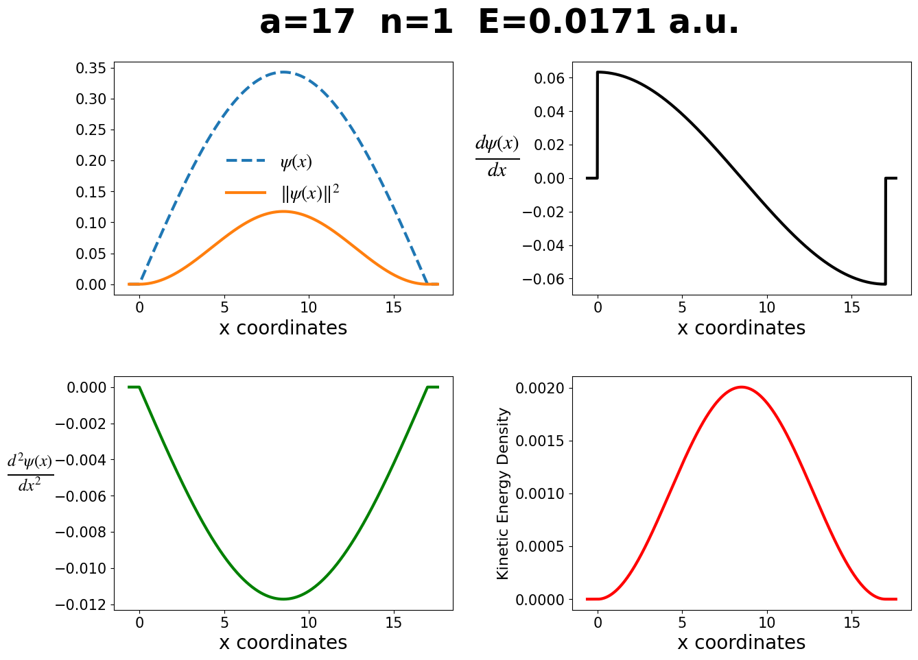
Visualizing the Particle-in-a-Box Wavefunctions, Probabilities, etc.#

In the next code block, the wavefunction, probability density, derivative, second-derivative, and kinetic energy density for the particle-in-a-box are shown. Notice that the kinetic-energy-density is proportional to the probability density, and that the first and second derivatives are not zero at the edge of the box, but the wavefunction and probability density are. It’s useful to change the parameters in the below figures to build your intuition for the particle-in-a-box.

#This next bit of code makes the plots and prints out the energy
def make_plots(a, n):
    #check the computed values of the moments against the analytic formula
    energy = compute_energy(n, a)
    print(f"The energy computed directly is {energy:.5f}")
    # sample x coordinates
    x = np.arange(-0.6, a + 0.6, 0.01)

    # evaluate wave-function & probability
    wf = compute_wavefunction(x, n, a)
    pr = compute_probability(x, n, a)

    # evaluate 1st & 2nd derivative of wavefunction w.r.t. x
    d1 = compute_wavefunction_derivative(x, n, a, order=1)
    d2 = compute_wavefunction_derivative(x, n, a, order=2)

    # evaluate kinetic energy density
    kin = compute_kinetic_energy_density(x, n, a)
    #print("Integrate KED = ", trapz(kin, x))


    # set the size of the plot
    plt.rcParams['figure.figsize'] = [15, 10]
    plt.rcParams['font.family'] = 'DejaVu Sans'
    plt.rcParams['font.serif'] = ['Times New Roman']
    plt.rcParams['mathtext.fontset'] = 'stix'
    plt.rcParams['xtick.labelsize'] = 15
    plt.rcParams['ytick.labelsize'] = 15

    # define four subplots
    fig, ((ax1, ax2), (ax3, ax4)) = plt.subplots(2, 2)
    fig.suptitle(f'a={a}  n={n}  E={compute_energy(n, a):.4f} a.u.', fontsize=35, fontweight='bold')

    # plot 1
    ax1.plot(x, wf, linestyle='--', label=r'$\psi(x)$', linewidth=3)
    ax1.plot(x, pr, linestyle='-', label=r'$\|\psi(x)\|^2$', linewidth=3)
    ax1.legend(frameon=False, fontsize=20)
    ax1.set_xlabel('x coordinates', fontsize=20)

    # plot 2
    ax2.plot(x, d1, linewidth=3, c='k')
    ax2.set_xlabel('x coordinates', fontsize=20)
    ax2.set_ylabel(r'$\frac{d\psi(x)}{dx}$', fontsize=30, rotation=0, labelpad=25)

    # plot 3
    ax3.plot(x, d2, linewidth=3, c='g', )
    ax3.set_xlabel('x coordinates', fontsize=20)
    ax3.set_ylabel(r'$\frac{d^2\psi(x)}{dx^2}$', fontsize=25, rotation=0, labelpad=25)

    # plot 4
    ax4.plot(x, kin, linewidth=3, c='r')
    ax4.set_xlabel('x coordinates', fontsize=20)
    ax4.set_ylabel('Kinetic Energy Density', fontsize=16)

    # adjust spacing between plots
    plt.subplots_adjust(left=0.125,
                    bottom=0.1, 
                    right=0.9, 
                    top=0.9, 
                    wspace=0.35, 
                    hspace=0.35)
    #Show Plot
    plt.show()
    
    
#Principle quantum number slider:
n = 1

#Box length slider:
a = 1


make_plots(a, n)

The energy computed directly is 4.93480

_images/98add1be76b2e3121f3acb5fb17bc65eaf08b70178c5c1682797566ae79ac20e.png

🪞 Self-Reflection#

Can you think of other physical or chemical systems where the particle-in-a-box Hamiltonian would be appropriate?
Can you think of another property density, besides the kinetic energy density, that cannot be uniquely defined in quantum mechanics?

🤔 Thought-Provoking Questions#

How would the wavefunction and ground-state energy change if you made a small change in the particle-in-a-box Hamiltonian, so that the right-hand-side of the box was a little higher than the left-hand-side?
Any system with a zero-point energy of zero is classical. Why?
How would you compute the probability of observing an electron at the center of a box if the box contained 2 electrons? If it contained 4 electrons? If it contained 8 electrons? The probability of observing an electron at the center of a box with 3 electrons is sometimes lower than the probability of observing an electron at the center of a box with 2 electrons. Why?
Demonstrate that the kinetic energy operator is linear and Hermitian.
What is the lowest-energy excitation energy for the particle-in-a-box?
Suppose you wanted to design a one-dimensional box containing a single electron that absorbed blue light? How long would the box be?

❓ Knowledge Tests#

Questions about the Particle-in-a-Box and related concepts. GitHub Classroom Link

👩🏽‍💻 Assignments#

Compute and understand expectation values by computing moments of the particle-in-a-box assignment. [Github classroom link]https://classroom.github.com/a/9yzWI5Vt.
This assignment on the sudden approximation provides an introduction to time-dependent phenomena. Github classroom link.

🔁 Recapitulation#

Write the Hamiltonian, time-independent Schrödinger equation, eigenfunctions, and eigenvalues for the one-dimensional particle in a box.
Play around with the eigenfunctions and eigenenergies of the particle-in-a-box to build intuition for them.
How would you compute the uncertainty in \(x^4\)?
Practice your calculus by explicitly computing, using integration by parts, \(\langle x \rangle\) and \(\langle x^2 \rangle\). This can be implemented in a Jupyter notebook.

🔮 Next Up…#

Postulates of Quantum Mechanics
Multielectron particle-in-a-box.
Multidimensional particle-in-a-box.
Harmonic Oscillator

📚 References#

My favorite sources for this material are:

Randy’s book has an excellent treatment of the particle-in-a-box model, including several extensions to the material covered here. (Chapter 3)
Also see my (pdf) class notes.
Also see my notes on the mathematical structure of quantum mechanics.
Davit Potoyan’s Jupyter-book covers the particle-in-a-box in chapter 4 are especially relevant here.
D. A. MacQuarrie, Quantum Chemistry (University Science Books, Mill Valley California, 1983)
An excellent explanation of the link to the spectrum of cyanine dyes
Chemistry Libre Text: one dimensional and multi-dimensional
McQuarrie and Simon summary

There are also some excellent wikipedia articles: