6. Multi-dimensional Particle-in-a-Box#
🥅 Learning Objectives#
Hamiltonian for a two-dimensional particle-in-a-box
Hamiltonian for a three-dimensional particle-in-a-box
Hamiltonian for a 3-dimensional spherical box
Separation of variables
Solutions for the 2- and 3- dimensional particle-in-a-box (rectangular)
Solutions for the 3-dimensional particle in a box (spherical)
Expectation values
The 2-Dimensional Particle-in-a-Box#
 We have treated the particle in a one-dimensional box, where the (time-independent) Schrödinger equation was:
where
However, electrons really move in three dimensions. However, just as sometimes electrons are (essentially) confined to one dimension, sometimes they are effectively confined to two dimensions. If the confinement is to a rectangle with side-widths \(a_x\) and \(a_y\), then the Schrödinger equation is:
where
The first thing to notice is that there are now two quantum numbers, \(n_x\) and \(n_y\).
The number of quantum numbers that are needed to label the state of a system is equal to its dimensionality.
The second thing to notice is that the Hamiltonian in this Schrödinger equation can be written as the sum of two Hamiltonians,
where
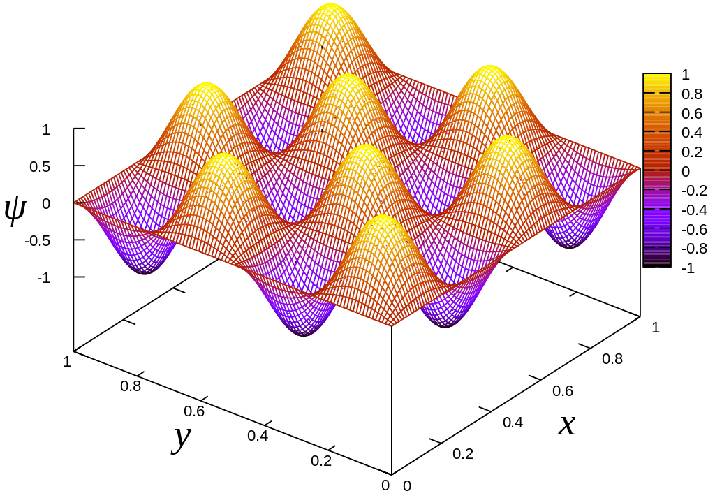
By the same logic as we used for the 1-dimensional particle in a box, we can deduce that the ground-state wavefunction for an electron in a rectangular box is:
The corresponding energy is thus:
📝 Exercise: Verify the above equation for the energy eigenvalues of a particle confined to a rectangular box.#
Separation of Variables#
The preceding solution is a very special case of a general approach called separation of variables.
Given a \(D\)-dimensional Hamiltonian that is a sum of independent terms,
where the solutions to the individual Schrödinger equations are known:
the solution to the \(D\)-dimensional Schrödinger equation is
where the \(D\)-dimensional eigenfunctions are products of the Schrödinger equations of the individual terms
and the \(D\)-dimensional eigenvalues are sums of the eigenvalues of the individual terms,
This expression can be verified by direct substitution. Interpretatively, in a Hamiltonian with the form
the coordinates \(x_1,x_2,\ldots,x_D\) are all independent, because there are no terms that couple them together in the Hamiltonian. This means that the probability of observing a particle with values \(x_1,x_2,\ldots,x_D\) are all independent. Recall that when probabilities are independent, they are multiplied together. E.g., if the probability that your impoverished professor will be paid today is independent of the probability that will rain today, then
Similarly, because \(x_1,x_2,\ldots,x_D\) are all independent,
Owing to the Born postulate, the probability distribution function for observing a particle at \(x_1,x_2,\ldots,x_D\) is the wavefunction squared, so
It is reassuring that the separation-of-independent-variables solution to the \(D\)-dimensional Schrödinger equation reproduces this intuitive conclusion.
📝 Exercise: By direct substitution, verify that the above expressions for the eigenvalues and eigenvectors of a Hamiltonian-sum are correct.#
📝 Exercise: Write the Time-Dependent Schrödinger equation for one particle, in three dimensions, confined by the time-dependent potential \(V(x,y,z,t)\).#
Degenerate States#
When two quantum states have the same energy, they are said to be degenerate. For example, for a square box, where \(a_x = a_y = a\), the states with \(n_x=1; n_y=2\) and \(n_x=2;n_y=1\) are degenerate because:
This symmetry reflects physical symmetry, whereby the \(x\) and \(y\) coordinates are equivalent. The state with energy \(E=\frac{5h^2}{8ma^2}\) is said to be two-fold degenerate, or to have degeneracy of two.
For the particle in a square box, degeneracies of all levels exist. An example of a three-fold degeneracy is:
and an example of a four-fold degeneracy is:
It isn’t trivial to show that degeneracies of all orders are possible (it’s tied up in the theory of Diophantine equations), but perhaps it becomes plausible by giving an example with an eight-fold degeneracy:
Notice that all of these degeneracies are removed if the symmetry of the box is broken. For example, if a slight change of the box changes it from square to rectangular, \(a_x \rightarrow a_x + \delta x\), then the aforementioned states have different energies. This doesn’t mean, however, that rectangular boxes do not have degeneracies. If \(\tfrac{a_x}{a_y}\) is a rational number, \(\tfrac{p}{q}\), then there will be an accidental degeneracies when \(n_x\) is divisible by \(p\) and \(n_y\) is divisible by \(q\). For example, if \(a_x = 2a\) and \(a_y = 3a\) (so \(p=2\) and \(q=3\)), there is a degeneracy associated with
This is called an accidental degeneracy because it is not related to a symmetry of the system, like the \(x \sim y\) symmetry that induces the degeneracy in the case of particles in a square box.
Electrons in a 3-dimensional box (cuboid)#
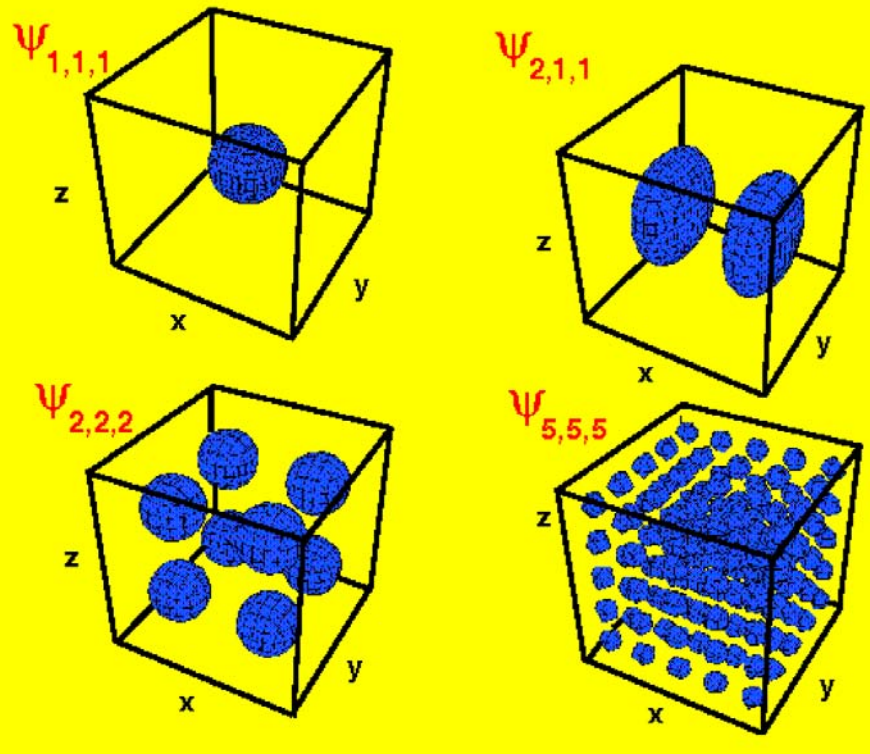
Suppose that particles are confined to a cuboid (or rectangular prism) with side-lengths \(a_x\), \(a_y\), and \(a_z\). Then the Schrödinger equation is:
where
There are three quantum numbers because the system is three-dimensional.
The three-dimensional second derivative is called the Laplacian, and is denoted
where
is the operator that defines the gradient vector. The 3-dimensional momentum operator is
which explains why the kinetic energy is given by
As with the 2-dimensional particle-in-a-rectangle, the 3-dimensional particle-in-a-cuboid can be solved by separation of variables. Rewriting the Schrödinger equation as:
where
By the same logic as we used for the 1-dimensional particle in a box, we can deduce that the ground-state wavefunction for an electron in a cuboid is:
The corresponding energy is thus:
As before, especially when there is symmetry, there are many degenerate states. For example, for a particle-in-a-cube, where \(a_x = a_y = a_z = a\), the first excited state is three-fold degenerate since:
There are other states of even higher degeneracy. For example, there is a twelve-fold degenerate state:
📝 Exercise: Verify the expressions for the eigenvalues and eigenvectors of a particle in a cuboid.#
📝 Exercise: Construct an accidentally degenerate state for the particle-in-a-cuboid.#
(Hint: this is a lot easier than you may think.)
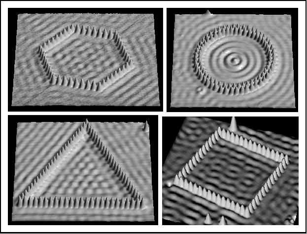
Particle-in-a-circle#
The Schrödinger equation for a particle confined to a circular disk.#
.jpg?raw=true)
What happens if instead of being confined to a rectangle or a cuboid, the electrons were confined to some other shape? For example, it is not uncommon to have electrons confined in a circular disk (quantum corral) or a sphere (quantum dot). It is relatively easy to write the Hamiltonian in these cases, but less easy to solve it because Cartesian (i.e., \(x,y,z\)) coordinates are less natural for these geometries.
The Schrödinger equation for a particle confined to a circular disk of radius \(a\) is:
where
However, it is more useful to write this in polar coordinates (i.e., \(r,\theta\)):
because the potential depends only on the distance from the center of the system,
where
The Schrödinger Equation in Polar Coordinates#
In order to solve this Schrödinger equation, we need to rewrite the Laplacian, \(\nabla^2 = \frac{d^2}{dx^2} + \frac{d^2}{dy^2}\) in polar coordinates. Deriving the Laplacian in alternative coordinate systems is a standard (and tedious) exercise that you hopefully saw in your calculus class. (If not, cf. wikipedia or this meticulous derivation.) The result is that:
The resulting Schrödinger equation is,
This looks like it might be amenable to solution by separation of variables insofar as the potential doesn’t compute the radial and angular positions of the particles, and the kinetic energy doesn’t couple the particles angular and radial momenta (i.e., the derivatives). So we propose the solution \(\psi(r,\theta) = R(r) \Theta(\theta)\). Substituting this into the Schrödinger equation, we obtain:
Dividing both sides by \(R(r) \Theta(\theta)\) and multiplying both sides by \(r^2\) we obtain:
The left-hand-side depends only on \(r\) and the right-hand-side depends only on \(\theta\); this can only be true for all \(r\) and all \(\theta\) if both sides are equal to the same constant. This problem can therefore be solved by separation of variables, though it is a slightly different form from the one we considered previously.
The Angular Schrödinger equation in Polar Coordinates#
To find the solution, we first solve the set the right-hand-side equal to a constant, which gives a 1-dimensional Schrödinger equations for the angular motion of the particle around the circle,
This equation is identical to the particle-in-a-box, and has (unnormalized) solutions
where \(l\) must be an integer because otherwise the fact the periodicity of the wavefunction (i.e., that \(\Theta_l(\theta) = \Theta_l(\theta + 2 k \pi)\) for any integer \(k\)) is not achieved. Using the expression for \(\Theta_l(\theta)\), the angular kinetic energy of the particle in a circle is seen to be:
The Radial Schrödinger equation in Polar Coordinates#
Inserting the results for the angular wavefunction into the Schrödinger equation, we obtain
which can be rearranged into the radial Schrödinger equation,
Notice that the radial eigenfunctions, \(R_{n,l}(r)\), and the energy eigenvalues, \(E_{n,l}\), depend on the angular motion of the particle, as quantized by \(l\). The term \(\frac{\hbar^2 l^2}{2mr^2}\) is exactly the centrifugal potential, indicating that it takes energy to hold a rotating particle in an orbit with radius \(r\), and that the potential energy that is required grows with \(r^{-2}\). Notice also that no assumptions have been made about the nature of the circular potential, \(V(r)\). The preceding analysis holds for any circular-symmetric potential.
The Radial Schrödinger Equation for a Particle Confined to a Circular Disk#
For the circular disk, where
it is somewhat more convenient to rewrite the radial Schrödinger equation as a homogeneous linear differential equation
Using the specific form of the equation, we have that, for \(0 \lt r \lt a\),
While this equation can be solved by the usual methods, that is beyond the scope of this course. However, we recognize that this equation is strongly resembles Bessel’s differential equation,
The solutions to Bessel’s equation are called the Bessel functions of the first kind and denoted, \(J_{\alpha}(r)\). However, the radial wavefunction must vanish at the edge of the disk, \(R_{n,l}(a) = 0\), and the Bessel functions generally do not satisfy this requirement. Recall that the boundary condition in the 1-dimensional particle in a box was satisfied by moving from the generic solution, \(\psi(x) \propto \sin(x)\) to the scaled solution, \(\psi(x) \propto \sin(k x)\), where \(k=\tfrac{2 \pi}{a}\) was chosen to satisfy the boundary condition. Similarly, we write the solutions as \(R_{n,l}(r) \propto J_l(kr)\). Substituting this form into the Schrödinger equation and using the fact that:
we have
Referring back to the Bessel equation, it is clear that this equation is satisfied when
or, equivalently,
where \(k\) is chosen so that \(J_l(ka) = 0\). If we label the zeros of the Bessel functions,
then
and the energies of the particle-in-a-disk are
and the eigenfunctions of the particle-in-a-disk are:

Eigenvalues and Eigenfunctions for a Particle Confined to a Circular Disk#
The energies of a particle confined to a circular disk of radius \(a\) are:
and its eigenfunctions are:
where \(x_{n,l}\) are the zeros of the Bessel function, \(J_l(x_{n,l}) = 0\). The first zero is \(x_{1,0} = 2.4048\). These solutions are exactly the resonant energies and modes that are associated with the vibration of a circular drum whose membrane has uniform thickness/density.
You can find elegant video animations of the eigenvectors of the particle-in-a-circle at the following links:
Interactive Demonstration of the States of a Particle-in-a-Circular-Disk
Movie animation of the quantum states of a particle-in-a-circular-disk
A subtle result, originally proposed by Bourget, is that no two Bessel functions ever have the same zeros, which means that the values of \(\{x_{n,l} \}\) are all distinct. A corollary of this is that eigenvalues of the particle confined to a circular disk are either nondegenerate (\(l=0\)) or doubly degenerate (\(|l| \ge 1\)). There are no accidental degeneracies for a particle in a circular disk.
The energies of an electron confined to a circular disk with radius \(a\) Bohr are:
The following code block computes these energies.
from scipy import constants
from scipy import special

import mpmath
# Define a function for the energy (in a.u.) of a particle in a circular disk
# with length a, principle quantum number n, and angular quantum number l
# The length is input in Bohr (atomic units).
def compute_energy_disk(n, l, a):
    "Compute 1-dimensional particle-in-a-spherical-ball energy."
    #Compute the first n zeros of the Bessel function
    zeros = special.jn_zeros(l,n)
    #Compute the energy from the n-th zero.
    return  (zeros[-1])**2/ (2 * a**2)

#This next bit of code just prints out the energy in atomic units
def print_energy_disk(a, n, l):
    print(f'The energy of an electron confined to a disk with radius {a:.2f} a.u.,'
       f' principle quantum number {n}, and angular quantum number {l}'
       f' is {compute_energy_disk(n, l, a):.3f} a.u..')

print_energy_disk(a, n, l)
---------------------------------------------------------------------------
NameError                                 Traceback (most recent call last)
Cell In[2], line 17
     13     print(f'The energy of an electron confined to a disk with radius {a:.2f} a.u.,'
     14        f' principle quantum number {n}, and angular quantum number {l}'
     15        f' is {compute_energy_disk(n, l, a):.3f} a.u..')
     16
---> 17 print_energy_disk(a, n, l)

NameError: name 'a' is not defined
Particle-in-a-Spherical Ball#
The Schrödinger equation for a particle confined to a spherical ball#

The final model we will consider for now is a particle confined to a spherical ball with radius \(a\),
where
However, it is more useful to write this in spherical polar coordinates (i.e., \(r,\theta, \phi\)):
because the potential depends only on the distance from the center of the system,
where
The Schrödinger Equation in Spherical Coordinates#
In order to solve the Schrödinger equation for a particle in a spherical ball, we need to rewrite the Laplacian, \(\nabla^2 = \frac{d^2}{dx^2} + \frac{d^2}{dy^2} + \frac{d^2}{dz^2}\) in polar coordinates. A meticulous derivation of the Laplacian and its eigenfunctions The result is that:
which can be rewritten in a more familiar form as:
Inserting this into the Schrödinger equation for a particle confined to a spherical potential, \(V(r)\), one has:
The solutions of the Schrödinger equation are characterized by three quantum numbers because this equation is 3-dimensional.
Recall that the classical equation for the kinetic energy of a set of points rotating around the origin, in spherical coordinates, is:
where \(p_{r,i}\) and \(\mathbf{L}_i\) are the radial and angular momenta of the \(i^{\text{th}}\) particle, respectively. It’s apparent, then, that the quantum-mechanical operator for the square of the angular momentum is:
The Schrödinger equation for a spherically-symmetric system is thus,
The Angular Wavefunction in Spherical Coordinates#

The Schrödinger equation for a spherically-symmetric system can be solved by separation of variables. If one compares to the result in polar coordinates, it is already clear that the angular wavefunction has the form \(\Theta(\theta,\phi) = P(\theta)e^{im_l\phi}\). From this starting point we could deduce the eigenfunctions of \(\hat{L}^2\), but instead we will just present the eigenfunctions and eigenvalues,
The functions \(Y_l^{m_l} (\theta, \phi)\) are called spherical harmonics, and they are the fundamental vibrational modes of the surface of a spherical membrane. Note that these functions resemble s-orbitals (\(l=0\)), p-orbitals (\(l=1\)), d-orbitals (\(l=2\)), etc., and that the number of choices for \(m_l\), \(2l+1\), is equal to the number of \(l\)-type orbitals.
The Radial Schrödinger equation in Spherical Coordinates#
Using separation of variables, we write the wavefunction as:
Inserting this expression into the Schrödinger equation, and exploiting the fact that the spherical harmonics are eigenfunctions of \(\hat{L}^2\), one obtains the radial Schrödinger equation:
Inside the sphere, \(V(r) = 0\). Rearranging the radial Schrödinger equation for the interior of the sphere as a homogeneous linear differential equation,
This equation strongly resembles the differential equations satisfied by the spherical Bessel functions, \(j_l(x)\)
The spherical Bessel functions are eigenfunctions for the particle-in-a-spherical-ball, but do not satisfy the boundary condition that the wavefunction be zero on the sphere, \(R_{n,l}(a) = 0\). To satisfy this constraint, we propose
Using this form in the radial Schrödinger equation, we have
Referring back to the differential equation satisfied by the spherical Bessel functions, it is clear that this equation is satisfied when
or, equivalently,
where \(k\) is chosen so that \(j_l(ka) = 0\). If we label the zeros of the spherical Bessel functions,
then
and the energies of the particle-in-a-ball are
and the eigenfunctions of the particle-in-a-ball are:
Notice that the eigenenergies have the same form as those in the particle-in-a-disk and even the same as those for a particle-in-a-one-dimensional-box; the only difference is the identity of the function whose zeros we are considering.
📝 Exercise: Use the equation for the zeros of \(\sin x\) to write the wavefunction and energy for the one-dimensional particle-in-a-box in a form similar to the expressions for the particle-in-a-disk and the particle-in-a-sphere.#
Solutions to the Schrödinger Equation for a Particle Confined to a Spherical Ball#
 The energies of a particle confined to a spherical ball of radius \(a\) are:
and its eigenfunctions are:
where \(y_{n,l}\) are the zeros of the spherical Bessel function, \(j_l(y_{n,l}) = 0\). The first spherical Bessel function, which corresponds to s-like solutions (\(l=0\)), is
and so
This gives explicit and useful expressions for the \(l=0\) wavefunctions and energies,
and its eigenfunctions are:
Notice that the \(l=0\) energies are the same as in the one-dimensional particle-in-a-box and the eigenfunctions are very similar.
In atomic units, the energies of an electron confined to a spherical ball with radius \(a\) Bohr are:
The following code block computes these energies. It uses the relationship between the spherical Bessel functions and the ordinary Bessel functions,
which indicates that the zeros of \(j_l(x)\) and \(J_{l+\tfrac{1}{2}}(x)\) occur the same places.
# Define a function for the energy (in a.u.) of a particle in a spherical ball
# with length a, principle quantum number n, and angular quantum number l
# The length is input in Bohr (atomic units).
def compute_energy_ball(n, l, a):
    "Compute 1-dimensional particle-in-a-spherical-ball energy."
    #Compute the energy from the n-th zero.
    return float((mpmath.besseljzero(l+0.5,n))**2/ (2 * a**2))

#This next bit of code just prints out the energy in atomic units
def print_energy_ball(a, n, l):
    print(f'The energy of an electron confined to a ball with radius {a:.2f} a.u.,'
       f' principle quantum number {n}, and angular quantum number {l}'
       f' is {compute_energy_ball(n, l, a):5.2f} a.u..')

print_energy_ball(a, n, l)
The energy of an electron confined to a ball with radius 1.00 a.u., principle quantum number 1, and angular quantum number 0 is 4.93 a.u..
📝 Exercise: For the hydrogen atom, the 2s orbital (\(n=2\), \(l=0\)) and 2p orbitals (\(n=2\),\(l=1\),\(m_l=-1,0,1\)) have the same energy. Is this true for the particle-in-a-ball?#
🪞 Self-Reflection#
Can you think of other physical or chemical systems where a multi-dimensional particle-in-a-box Hamiltonian would be appropriate? What shape would the box be?
Can you think of another chemical system where separation of variables would be useful?
Explain why separation of variables is consistent with the Born Postulate that the square-magnitude of a particle’s wavefunction is the probability distribution function for the particle.
What is the expression for the zero-point energy and ground-state wavefunction of an electron in a 4-dimensional box? Can you identify some states of the 4-dimensional box with especially high degeneracy?
What is the degeneracy of the k-th excited state of a particle confined to a circular disk? What is the degeneracy of the k-th excited state of a particle confined in a spherical ball?
Write a Python function that computes the normalization constant for the particle-in-a-disk and the particle-in-a-sphere.
🤔 Thought-Provoking Questions#
How would you write the Hamiltonian for two electrons confined to a box? Could you solve this system with separation of variables? Why or why not?
Write the time-independent Schrödinger equation for an electron in an cylindrical box. What are its eigenfunctions and eigenvalues?
What would the time-independent Schrödinger equation for electrons in an elliptical box look like? (You may find it useful to reference elliptical and ellipsoidal coordinates.
Construct an example of a four-fold accidental degeneracy for a particle in a 2-dimensional rectangular (not square!) box.
If there is any degenerate state (either accidental or due to symmetry) for the multi-dimensional particle-in-a-box, then there are always an infinite number of other degenerate states. Why?
Consider an electron confined to a circular harmonic well, \(V(r) = k r^2\). What is the angular kinetic energy and angular wavefunction for this system?
🔁 Recapitulation#
Write the Hamiltonian, time-independent Schrödinger equation, eigenfunctions, and eigenvalues for two-dimensional and three-dimensional particles in a box.
What is the definition of degeneracy? How does an “accidental” degeneracy differ from an ordinary degeneracy?
What is the zero-point energy for an electron in a circle and an electron in a sphere?
What are the spherical harmonics?
Describe the technique of separation of variables? When can it be applied?
What is the Laplacian operator in Cartesian coordinates? In spherical coordinates?
What are boundary conditions and how are they important in quantum mechanics?
🔮 Next Up…#
1-electron atoms
Approximate methods for quantum mechanics
Multielectron particle-in-a-box
📚 References#
My favorite sources for this material are:
Randy’s book (See Chapter 3)
Also see my (pdf) class [notes] (PaulWAyers/IntroQChem).
Meticulous solution for a particle confined to a circular disk
General discussion of the particle-in-a-region, which is the same as the classical wave equation
There are also some excellent wikipedia articles: