3. From Newton to Schrödinger#
🥅 Learning Objectives#
To learn about the historical origins of quantum mechanics.
To introduce wave-particle duality and key concepts like the
Planck-Einstein relation for the energy of a photon
Einstein-Compton-De Broglie relation between momentum and wavelength
quantization of energy levels
To introduce the Schrödinger equation and the probabilistic interpretation thereof.
What is Quantum Mechanics#
Starting in the late 1800’s, experimental physicists began to make observations that challenged the “classical” equations of physics. What emerged was quantum mechanics. Quantum mechanics unifies and supersedes the theories of classical Newtonian mechanics and classical Maxwellian electromagnetism.
In classical physics, radiation and matter are inherently different: radiation and matter are governed by different physical laws and modeled with different equations. Quantum mechanics abolishes the inherent difference between radiation and matter. Radiation—e.g., light—has properties (a well-defined energy and momentum) that are associated with matter. Matter—e.g., an electron—has properties (a wavelength) that are associated with radiation.
The wave-like-ness of matter immediately leads to something called quantization. Matter is “chunky.” There is no such thing as “half an electron.” One always has an integer number of elementary particles. So if I give you a system containing some number of electrons, you can safely say that the total mass of the system is
where \(m_e\) is the mass of the electron and \(n_e\) is a nonnegative integer. Using mass-energy equivalence, this means that the energy of these electrons should also be discrete
where \(c\) is the speed of light.
Waves, however do not seem to be “chunky”. If I want to put more energy into a wave, I can increase its amplitude or increase its frequency (by an noninteger amount). So it would seem possible to make waves with any amount of energy. It was Max Planck, in 1900, that proposed that there should also be a “quantization” of radiation, and that radiation should come in integer chunks, with the energy proportional to the frequency of the radiation:
The proportional constant is called Planck’s constant:
where
Planck’s constant is very small, which explains why electromagnetic radiation does not seem to be “chunky” in everyday life. Similarly, the masses and charges of elementary particles are very small, which is why Newtonian mechanics is accurate enough to describe macroscopic phenomena. However, it is essential to include quantum effects when we deal with particles with very little mass (e.g., electrons).
Planck proposed the quantization of radiation as a mathematical trick to provide a model for blackbody radiation. In 1905, Einstein interpreted this trick in the most literal possible way, proposing the quantization of light. This interpretation led to an interpretation of the photoelectric effect, which eventually earned Einstein the Nobel Prize in Physics. Planck also won the Nobel Prize in physics.

How was Quantum Mechanics Discovered?#
It is impossible to fully explain the historical foundations of quantum mechanics in a course like this one. Instead, I will try to give you a very brief overview of some key experiments that changed physics.
Black-body Radiation#
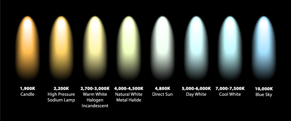
An inflammable object that absorbs all incident light, but does not transmit or reflect light, is called a black body. Because it is totally opaque and absorbs all light that falls upon it, a black body at zero Kelvin is the very definition of black. However, when you heat a blackbody, it glows. A good (but not perfect) example of a black body is a red-hot poker. An even better example is the sun. Blackbody radiation has been observed by humans for millennia (or even longer): lava flows, molten glass, molten metal, and many other materials can be considered blackbodies. So it was extremely embarrassing to 19th-century physicists that they could not predict the spectrum—that is, which wavelengths of light occur with what intensity—of a blackbody.
In principle the spectrum of a black body should be easy to describe with classical statistical mechanics. However, classical statistical mechanics predicted that most of the light emitted would have a very short wavelength, the so-called “ultraviolet catastrophe.” Planck suggested that the vibrations of atoms in a black body, and ergo the light emitted therefrom, was quantized into chunks. Planck understood that his result was significant, but he still thought of it as a mathematical trick.
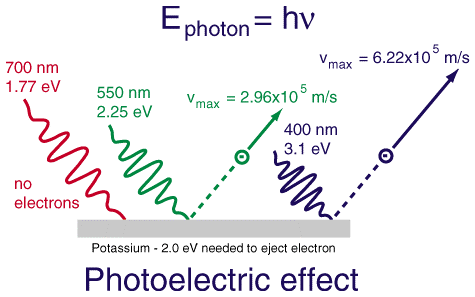
Photoelectric Effect#
When one shines light on a metal surface, one observes that if the light has a low enough frequency (long enough wavelength), then no electrons escape from the surface. This holds (to an excellent approximation) no matter how intense the light is. However, with a sufficiently high frequency (short enough wavelength), electrons will start to escape from the surface. Importantly, the maximum kinetic energy of the electrons escaping from the surface grows as the frequency of the light increases, and the number of electrons escaping from the surface grows as the intensity of the light increases. But increasing the intensity of the light does not increase the maximum kinetic energy of the emitted electrons, nor does increasing the frequency of the light increase the number of electrons emitted.
Einstein decided to take Planck’s mathematical expression at face value, and interpret light as coming in chunks called photons, with energy given by Planck’s expression:
This allowed him to describe the photoelectric effect. Specifically, whenever \(h \nu \) was less than a threshold value for the substance called its work function, \(W\), no electrons would be emitted. (The work function can be thought of as the “ionization potential” for a metal.) But when \(h \nu > W\), then photons had enough energy to remove an electron from the metal, and the surplus energy from the photon could be imparted to the electron as kinetic energy. Ergo
As the light becomes more intense, the number of photons increases and the number of electrons emitted increases but, unless the light is very, very, very intense, the maximum kinetic energy of the electrons is left unaltered.

Compton Effect#
When you shine light on an (isolated) electron sitting at rest, sometimes the light scatters inelastically—that is the emitted light has a lower frequency than the incident light. The change in energy between the incident and emitted light is manifest in the kinetic energy of the electron. However, it’s observed that the electron does not move in an arbitrary direction, but instead moves in the direction that would be expected if a photon were a classical particle moving at the speed of light with effective mass \(m_{ph,\text{eff}} = \tfrac{h \nu}{c^2}\). Note that the photon does not actually have mass. However, the photon does have momentum, which explains the inelastic scattering result. The formula is derived by assuming that one can set the rest-mass-energy expression, \(E = m c^2\), to the Planck relation for the energy of a photon. Then
and the momentum of the photon would be its effective mass times its speed, \(c\):
Recall that the wavelength, \(\lambda\), and frequency, \(\nu\) of light are related according to the relation
This means that the momentum of light can be expressed as
This is called the De Broglie relation. One of the key results of quantum mechanics is that the De Broglie relation holds for both waves (photons) and particles.

Davisson-Germer Experiment#
Based on the results of Compton and De Broglie, one should expect that a beam of electrons should diffract, with patterns of constructive and deconstructive interference, according to their wavelength. The Davisson-Germer experiment confirmed this, showing that electrons (particles) can constructively and deconstructively interfere like waves.
Rydberg Formula#
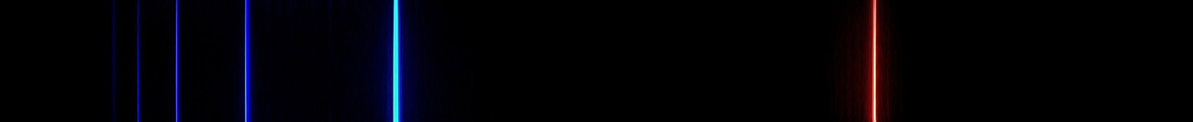
By the late 1800s, it was known that when a dilute atomic gas was heated, it did not emit as a black body, but only at certain characteristic wavelengths. Rydberg managed to describe the specific wavelengths of the emission by the empirical formula
where \(n\) and \(m\) are positive integers: \(n,m = 1,2,3,4,\ldots\). Recalling the link between frequency and wavelength, \(\nu = \tfrac{c}{\lambda}\) and the Planck-Einstein relation for the energy of a photon,
This suggests that photons are associated with transitions between energy levels that are labelled by indices, suggesting that the electronic energy levels of atoms are not arbitrary, but only have certain, quantized, values. The Rydberg formula is accurate for all one-electron atoms (at least until relativistic effects become nonneglible). It is also valid for highly-excited states (so-called Rydberg excitations) of many-electron atoms, where a single highly-excited electron is much further from the nucleus than the other electrons.
Wave-Particle Duality#
It seems as though we must use sometimes the one theory and sometimes the other, while at times we may use either. We are faced with a new kind of difficulty. We have two contradictory pictures of reality; separately neither of them fully explains the phenomena … but together they do. - Albert Einstein
The previous experiments, among many others, established that particles like electrons have wave-like properties, that electromagnetic radiation is composed of discrete photons with particle-like momentum and energy. The fact particles possess wave-like properties and waves provide particle-like properties is called wave-particle duality: there is only one type of “stuff” in the universe and that stuff is “chunky” (like particles) and can constructively and deconstructively interfere (like waves). Moreover, the energies of atoms and molecules are quantized, having only specific discrete values.
📝 Exercise: Suppose you are given a photon with an energy of 2 eV. What is its momentum in \(\frac{\text{m} \cdot \text{kg}}{\text{s}}\)? What is its frequency in Hz?#
📝 Exercise: What is the momentum and energy of a photon with angular wavenumber \(k=\frac{2\pi}{\lambda} = 10^7 \text{m}^{-1}\)? Give your answer in SI units.#
The Schrödinger Equation#
It seems that, in physics, the more we learn, the simpler things become. We used to believe that there were two types of things, “particles” (matter) and “waves” (radiation). Now we understand that there is really only one type of entity, perhaps call it a wavicle if you must give it a name. Electromagnetic radiation comes in discrete chunks (photons) just like particles (e.g., electrons). Photons and particles have position(ish), momentum(ish), and energy(ish), just like classical particles of matter; both also can manifest constructive and deconstructive interference, just like classical waves. The difference between matter and radiation is merely one of perspective.
In 1925-26, Heisenberg and Schrödinger, working independently, built mathematical frameworks to describe the wave-particle duality of quantum particles. Nowadays we usually (except sometimes in spectroscopy) prefer Schrödinger’s formulation. We will discuss the Schrödinger equation in more detail in the next unit, but for now it is worth merely comparing it to other equations from classical mechanics and classical electromagnetism, just to intuitively show how it encapsulates wave-particle duality. Of course, a more rigorous justification for the Schrödinger equation is beyond the scope of this course.
For simplicity, we will only consider systems in one dimension.
Wave Equation (classical electromagnetism)
\[ \frac{d^2u(x,t)}{dt^2} = c^2 \frac{d^2u(x,t)}{dx^2} \]
Hamilton-Jacobi Equation (classical mechanics)
\[ -\frac{dS(x,t)}{dt} = H \]
where \(H = T + V\) is the sum of the kinetic energy, \(T\), and the potential energy, \(V\), written as a function of \(S\), \(x\), and \(t\). In the simplest case, one has:
\[ -\frac{dS(x,t)}{dt} = \left( \frac{1}{2m} \frac{dS(x,t)}{dx} \cdot \frac{dS(x,t)}{dx} + V(x,t) \right) \]
because the momentum can be identified as \(p(x,t) = \tfrac{dS(x,t)}{dx} \).
Schrödinger Equation (quantum mechanics)
\[ \frac{i h}{2 \pi} \frac{d \Psi(x,t)}{dt} = \left( -\frac{h^2}{2m (2 \pi)^2 } \frac{d^2 \Psi(x,t)}{dx^2} + V(x,t)\Psi(x,t) \right) \]The solution, \(\Psi(x,t)\) to the Schrödinger equation is called the wavefunction. A key postulate of quantum mechanics is that the wavefunction contains all the information needed to fully specify the observable properties of a quantum system.
All three equations have strong resemblance. But, in particular, the Schrödinger equation and the Hamilton-Jacobi equation are consistent with each other. Suppose one uses the wavefunction ansatz,
where \(\psi_0(x,t)\) and \(S(x,t)\) are, without loss of generality, assumed to be real-valued functions. We will insert this expression into the Schrödinger equation, but first it is useful to define the quantity
One then can rewrite the wavefunction and the Schrödinger equation without the pesky factors of \(2 \pi\), respectively,
Inserting the wavefunction into the Schrödinger equation, the left-hand-side is
and the right-hand-side is
Inserting these equations into the Schrödinger equation and dividing through by \(e^{\frac{i S(x,t)}{\hbar}}\) gives:
The real and imaginary parts of this equation must be separately equal to each other. The real part of the equation is
Dividing both sides by \(\psi_0(x,t)\) and taking the classical limit, where \(\hbar \rightarrow 0\), gives back the Hamilton-Jacobi equation,
The imaginary part of the equation is:
We notice that this expression is zero in the classical limit. Dividing through by \(\hbar\) and using the chain rule, \(\frac{d \left(\psi_0(x,t)\right)^2}{dt} = 2 \psi_0(x,t) \frac{d \psi_0(x,t)}{dt}\), we can rewrite this expression as
This expression resembles the equation of continuity from classical physics,
where \(v(x,t)\) is the velocity and \(\rho(x,t)\) is the density, the probability of observing a particle at the point \(x\) and the time \(t\). This (re)confirms that \(\nabla S\) is an expression for the momentum, and suggests that
is an expression for the probability of observing a particle at a point in space. The identification of the square-magnitude of the quantum-mechanical wavefunction with probability is called the Born postulate.
In the end, the Schrödinger equation was not accepted because of its mathematical elegance, but because it worked to accurately describe key phenomena. In fact, as we shall see, the (originally empirical) Rydberg formula can be easily justified using the Schrödinger equation.
We can rationalize the form of the quantum mechanical momentum operator, \(\hat{p} = -i \hbar \frac{d}{dx} \) , by a similar argument. Applying the hypothesized momentum operator to the wavefunction, one obtains:
This indicates that the quantum-mechanical momentum operator is consistent with the classical expression for the momentum, to which it reduces in the classical limit where \(\hbar \rightarrow 0\).
🪞 Self-Reflection#
Imagine you were assigned to describe Quantum Mechanics to a room full of irascible tweens.
How would you motivate them to be interested in quantum mechanics?
How would you describe wave-particle duality in a way they could understand?
❓ Knowledge Test#
This set of questions demonstrates the different types of knowledge-test questions that appear in the course, and how to solve them. GitHub Classroom Link
More questions, mostly about wave-particle duality. GitHub Classroom Link
🤔 Thought-Provoking Questions#
Is it possible for the wavelength of the scattered photon in Compton Scattering to be infinite? (I.e., could the photon be entirely absorbed?)
What are the units of the wavefunction?
🔁 Recapitulation#
What are the following phenomena/experiments/theories, and why were they important to the establishment of the quantum theory?
black-body radiation and the ultraviolet catastrophe
the photoelectric effect
Compton scattering
the Davisson-Germer experiment (and electron scattering/diffraction in general)
the spectral lines of one-electron atoms, and the Rydberg relation
What are the following key equations, and why are they important?
Planck-Einstein relation for the energy of a photon
De Broglie relation between momentum and wavelength
the Schrödinger equation
What is the quantum mechanical operator for the momentum of a particle?
List as many properties/characteristics of the wavefunction as you can.
🔮 Next Up…#
Motivate the time-dependent Schrödinger equation
Derive the time-independent Schrödinger equation
Explore the quantum-mechanical operator for momentum
Study simple one-dimensional Hamiltonians
📚 References#
My favorite sources for this material are:
R. Eisberg and R. Resnick, Quantum Physics of Atoms, Molecules, Solids, Nuclei, and Particles (Wiley, New York, 1974)
R. Dumont, An Emergent Reality, Part 2: Quantum Mechanics (Chapters 1 and 2).
Also see my (pdf) class notes.
The introductory material in Davit Potoyan’s Jupyter-book course is very good. Roughly chapters 1 and 2 are especially relevant here.
Some videos:
There are also some excellent wikipedia articles:
On General Quantum Mechanics
Black-Body Radiation
Electron/Particle Diffraction
Spectral lines in simple atoms
Schrödinger Equation